Jupyter Snippet SPL Lecture-6B-HPC
Jupyter Snippet SPL Lecture-6B-HPC
Lecture 6B - Tools for high-performance computing applications
J.R. Johansson (jrjohansson at gmail.com)
The latest version of this IPython notebook lecture is available at http://github.com/jrjohansson/scientific-python-lectures.
The other notebooks in this lecture series are indexed at http://jrjohansson.github.io.
%matplotlib inline
import matplotlib.pyplot as plt
multiprocessing
Python has a built-in process-based library for concurrent computing, called multiprocessing.
import multiprocessing
import os
import time
import numpy
def task(args):
    print("PID =", os.getpid(), ", args =", args)

    return os.getpid(), args
task("test")
PID = 28995 , args = test


(28995, 'test')
pool = multiprocessing.Pool(processes=4)
result = pool.map(task, [1,2,3,4,5,6,7,8])
PID = 29006 , args = 1
PID = 29009 , args = 4
PID = 29007 , args = 2
PID = 29008 , args = 3
PID = 29006 , args = 6
PID = 29009 , args = 5
PID = 29007 , args = 8
PID = 29008 , args = 7
result
[(29006, 1),
 (29007, 2),
 (29008, 3),
 (29009, 4),
 (29009, 5),
 (29006, 6),
 (29008, 7),
 (29007, 8)]
The multiprocessing package is very useful for highly parallel tasks that do not need to communicate with each other, other than when sending the initial data to the pool of processes and when and collecting the results.
IPython parallel
IPython includes a very interesting and versatile parallel computing environment, which is very easy to use. It builds on the concept of ipython engines and controllers, that one can connect to and submit tasks to. To get started using this framework for parallel computing, one first have to start up an IPython cluster of engines. The easiest way to do this is to use the ipcluster command,
$ ipcluster start -n 4
Or, alternatively, from the “Clusters” tab on the IPython notebook dashboard page. This will start 4 IPython engines on the current host, which is useful for multicore systems. It is also possible to setup IPython clusters that spans over many nodes in a computing cluster. For more information about possible use cases, see the official documentation Using IPython for parallel computing.
To use the IPython cluster in our Python programs or notebooks, we start by creating an instance of IPython.parallel.Client:
from IPython.parallel import Client
cli = Client()
Using the ‘ids’ attribute we can retreive a list of ids for the IPython engines in the cluster:
cli.ids
[0, 1, 2, 3]
Each of these engines are ready to execute tasks. We can selectively run code on individual engines:
def getpid():
    """ return the unique ID of the current process """
    import os
    return os.getpid()
# first try it on the notebook process
getpid()
28995
# run it on one of the engines
cli[0].apply_sync(getpid)
30181
# run it on ALL of the engines at the same time
cli[:].apply_sync(getpid)
[30181, 30182, 30183, 30185]
We can use this cluster of IPython engines to execute tasks in parallel. The easiest way to dispatch a function to different engines is to define the function with the decorator:
@view.parallel(block=True)
Here, view is supposed to be the engine pool which we want to dispatch the function (task). Once our function is defined this way we can dispatch it to the engine using the map method in the resulting class (in Python, a decorator is a language construct which automatically wraps the function into another function or a class).
To see how all this works, lets look at an example:
dview = cli[:]
@dview.parallel(block=True)
def dummy_task(delay):
    """ a dummy task that takes 'delay' seconds to finish """
    import os, time

    t0 = time.time()
    pid = os.getpid()
    time.sleep(delay)
    t1 = time.time()

    return [pid, t0, t1]
# generate random delay times for dummy tasks
delay_times = numpy.random.rand(4)
Now, to map the function dummy_task to the random delay time data, we use the map method in dummy_task:
dummy_task.map(delay_times)
[[30181, 1395044753.2096598, 1395044753.9150908],
 [30182, 1395044753.2084103, 1395044753.4959202],
 [30183, 1395044753.2113762, 1395044753.6453338],
 [30185, 1395044753.2130392, 1395044754.1905618]]
Let’s do the same thing again with many more tasks and visualize how these tasks are executed on different IPython engines:
def visualize_tasks(results):
    res = numpy.array(results)
    fig, ax = plt.subplots(figsize=(10, res.shape[1]))

    yticks = []
    yticklabels = []
    tmin = min(res[:,1])
    for n, pid in enumerate(numpy.unique(res[:,0])):
        yticks.append(n)
        yticklabels.append("%d" % pid)
        for m in numpy.where(res[:,0] == pid)[0]:
            ax.add_patch(plt.Rectangle((res[m,1] - tmin, n-0.25),
                         res[m,2] - res[m,1], 0.5, color="green", alpha=0.5))

    ax.set_ylim(-.5, n+.5)
    ax.set_xlim(0, max(res[:,2]) - tmin + 0.)
    ax.set_yticks(yticks)
    ax.set_yticklabels(yticklabels)
    ax.set_ylabel("PID")
    ax.set_xlabel("seconds")
delay_times = numpy.random.rand(64)
result = dummy_task.map(delay_times)
visualize_tasks(result)

That’s a nice and easy parallelization! We can see that we utilize all four engines quite well.
But one short coming so far is that the tasks are not load balanced, so one engine might be idle while others still have more tasks to work on.
However, the IPython parallel environment provides a number of alternative “views” of the engine cluster, and there is a view that provides load balancing as well (above we have used the “direct view”, which is why we called it “dview”).
To obtain a load balanced view we simply use the load_balanced_view method in the engine cluster client instance cli:
lbview = cli.load_balanced_view()
@lbview.parallel(block=True)
def dummy_task_load_balanced(delay):
    """ a dummy task that takes 'delay' seconds to finish """
    import os, time

    t0 = time.time()
    pid = os.getpid()
    time.sleep(delay)
    t1 = time.time()

    return [pid, t0, t1]
result = dummy_task_load_balanced.map(delay_times)
visualize_tasks(result)

In the example above we can see that the engine cluster is a bit more efficiently used, and the time to completion is shorter than in the previous example.
Further reading
There are many other ways to use the IPython parallel environment. The official documentation has a nice guide:
MPI
When more communication between processes is required, sophisticated solutions such as MPI and OpenMP are often needed. MPI is process based parallel processing library/protocol, and can be used in Python programs through the mpi4py package:
To use the mpi4py package we include MPI from mpi4py:
from mpi4py import MPI
A MPI python program must be started using the mpirun -n N command, where N is the number of processes that should be included in the process group.
Note that the IPython parallel enviroment also has support for MPI, but to begin with we will use mpi4py and the mpirun in the follow examples.
Example 1
%%file mpitest.py

from mpi4py import MPI

comm = MPI.COMM_WORLD
rank = comm.Get_rank()

if rank == 0:
   data = [1.0, 2.0, 3.0, 4.0]
   comm.send(data, dest=1, tag=11)
elif rank == 1:
   data = comm.recv(source=0, tag=11)

print "rank =", rank, ", data =", data
Overwriting mpitest.py
!mpirun -n 2 python mpitest.py
rank = 0 , data = [1.0, 2.0, 3.0, 4.0]
rank = 1 , data = [1.0, 2.0, 3.0, 4.0]
Example 2
Send a numpy array from one process to another:
%%file mpi-numpy-array.py

from mpi4py import MPI
import numpy

comm = MPI.COMM_WORLD
rank = comm.Get_rank()

if rank == 0:
   data = numpy.random.rand(10)
   comm.Send(data, dest=1, tag=13)
elif rank == 1:
   data = numpy.empty(10, dtype=numpy.float64)
   comm.Recv(data, source=0, tag=13)

print "rank =", rank, ", data =", data
Overwriting mpi-numpy-array.py
!mpirun -n 2 python mpi-numpy-array.py
rank = 0 , data = [ 0.71397658  0.37182268  0.25863587  0.08007216  0.50832534  0.80038331
  0.90613024  0.99535428  0.11717776  0.48353805]
rank = 1 , data = [ 0.71397658  0.37182268  0.25863587  0.08007216  0.50832534  0.80038331
  0.90613024  0.99535428  0.11717776  0.48353805]
Example 3: Matrix-vector multiplication
# prepare some random data
N = 16
A = numpy.random.rand(N, N)
numpy.save("random-matrix.npy", A)
x = numpy.random.rand(N)
numpy.save("random-vector.npy", x)
%%file mpi-matrix-vector.py

from mpi4py import MPI
import numpy

comm = MPI.COMM_WORLD
rank = comm.Get_rank()
p = comm.Get_size()

def matvec(comm, A, x):
    m = A.shape[0] / p
    y_part = numpy.dot(A[rank * m:(rank+1)*m], x)
    y = numpy.zeros_like(x)
    comm.Allgather([y_part,  MPI.DOUBLE], [y, MPI.DOUBLE])
    return y

A = numpy.load("random-matrix.npy")
x = numpy.load("random-vector.npy")
y_mpi = matvec(comm, A, x)

if rank == 0:
    y = numpy.dot(A, x)
    print(y_mpi)
    print "sum(y - y_mpi) =", (y - y_mpi).sum()
Overwriting mpi-matrix-vector.py
!mpirun -n 4 python mpi-matrix-vector.py
[ 6.40342716  3.62421625  3.42334637  3.99854639  4.95852419  6.13378754
  5.33319708  5.42803442  5.12403754  4.87891654  2.38660728  6.72030412
  4.05218475  3.37415974  3.90903001  5.82330226]
sum(y - y_mpi) = 0.0
Example 4: Sum of the elements in a vector
# prepare some random data
N = 128
a = numpy.random.rand(N)
numpy.save("random-vector.npy", a)
%%file mpi-psum.py

from mpi4py import MPI
import numpy as np

def psum(a):
    r = MPI.COMM_WORLD.Get_rank()
    size = MPI.COMM_WORLD.Get_size()
    m = len(a) / size
    locsum = np.sum(a[r*m:(r+1)*m])
    rcvBuf = np.array(0.0, 'd')
    MPI.COMM_WORLD.Allreduce([locsum, MPI.DOUBLE], [rcvBuf, MPI.DOUBLE], op=MPI.SUM)
    return rcvBuf

a = np.load("random-vector.npy")
s = psum(a)

if MPI.COMM_WORLD.Get_rank() == 0:
    print "sum =", s, ", numpy sum =", a.sum()
Overwriting mpi-psum.py
!mpirun -n 4 python mpi-psum.py
sum = 64.948311241 , numpy sum = 64.948311241
Further reading
OpenMP
What about OpenMP? OpenMP is a standard and widely used thread-based parallel API that unfortunaltely is not useful directly in Python. The reason is that the CPython implementation use a global interpreter lock, making it impossible to simultaneously run several Python threads. Threads are therefore not useful for parallel computing in Python, unless it is only used to wrap compiled code that do the OpenMP parallelization (Numpy can do something like that).
This is clearly a limitation in the Python interpreter, and as a consequence all parallelization in Python must use processes (not threads).
However, there is a way around this that is not that painful. When calling out to compiled code the GIL is released, and it is possible to write Python-like code in Cython where we can selectively release the GIL and do OpenMP computations.
N_core = multiprocessing.cpu_count()

print("This system has %d cores" % N_core)
This system has 12 cores
Here is a simple example that shows how OpenMP can be used via cython:
%load_ext cythonmagic
%%cython -f -c-fopenmp --link-args=-fopenmp -c-g

cimport cython
cimport numpy
from cython.parallel import prange, parallel
cimport openmp

def cy_openmp_test():

    cdef int n, N

    # release GIL so that we can use OpenMP
    with nogil, parallel():
        N = openmp.omp_get_num_threads()
        n = openmp.omp_get_thread_num()
        with gil:
            print("Number of threads %d: thread number %d" % (N, n))
cy_openmp_test()
Number of threads 12: thread number 0
Number of threads 12: thread number 10
Number of threads 12: thread number 8
Number of threads 12: thread number 4
Number of threads 12: thread number 7
Number of threads 12: thread number 3
Number of threads 12: thread number 2
Number of threads 12: thread number 1
Number of threads 12: thread number 11
Number of threads 12: thread number 9
Number of threads 12: thread number 5
Number of threads 12: thread number 6
Example: matrix vector multiplication
# prepare some random data
N = 4 * N_core

M = numpy.random.rand(N, N)
x = numpy.random.rand(N)
y = numpy.zeros_like(x)
Let’s first look at a simple implementation of matrix-vector multiplication in Cython:
%%cython

cimport cython
cimport numpy
import numpy

@cython.boundscheck(False)
@cython.wraparound(False)
def cy_matvec(numpy.ndarray[numpy.float64_t, ndim=2] M,
              numpy.ndarray[numpy.float64_t, ndim=1] x,
              numpy.ndarray[numpy.float64_t, ndim=1] y):

    cdef int i, j, n = len(x)

    for i from 0 <= i < n:
        for j from 0 <= j < n:
            y[i] += M[i, j] * x[j]

    return y
# check that we get the same results
y = numpy.zeros_like(x)
cy_matvec(M, x, y)
numpy.dot(M, x) - y
array([ 0.,  0.,  0.,  0.,  0.,  0.,  0.,  0.,  0.,  0.,  0.,  0.,  0.,
        0.,  0.,  0.,  0.,  0.,  0.,  0.,  0.,  0.,  0.,  0.,  0.,  0.,
        0.,  0.,  0.,  0.,  0.,  0.,  0.,  0.,  0.,  0.,  0.,  0.,  0.,
        0.,  0.,  0.,  0.,  0.,  0.,  0.,  0.,  0.])
%timeit numpy.dot(M, x)
100000 loops, best of 3: 2.93 µs per loop
%timeit cy_matvec(M, x, y)
100000 loops, best of 3: 5.4 µs per loop
The Cython implementation here is a bit slower than numpy.dot, but not by much, so if we can use multiple cores with OpenMP it should be possible to beat the performance of numpy.dot.
%%cython -f -c-fopenmp --link-args=-fopenmp -c-g

cimport cython
cimport numpy
from cython.parallel import parallel
cimport openmp

@cython.boundscheck(False)
@cython.wraparound(False)
def cy_matvec_omp(numpy.ndarray[numpy.float64_t, ndim=2] M,
                  numpy.ndarray[numpy.float64_t, ndim=1] x,
                  numpy.ndarray[numpy.float64_t, ndim=1] y):

    cdef int i, j, n = len(x), N, r, m

    # release GIL, so that we can use OpenMP
    with nogil, parallel():
        N = openmp.omp_get_num_threads()
        r = openmp.omp_get_thread_num()
        m = n / N

        for i from 0 <= i < m:
            for j from 0 <= j < n:
                y[r * m + i] += M[r * m + i, j] * x[j]

    return y
# check that we get the same results
y = numpy.zeros_like(x)
cy_matvec_omp(M, x, y)
numpy.dot(M, x) - y
array([ 0.,  0.,  0.,  0.,  0.,  0.,  0.,  0.,  0.,  0.,  0.,  0.,  0.,
        0.,  0.,  0.,  0.,  0.,  0.,  0.,  0.,  0.,  0.,  0.,  0.,  0.,
        0.,  0.,  0.,  0.,  0.,  0.,  0.,  0.,  0.,  0.,  0.,  0.,  0.,
        0.,  0.,  0.,  0.,  0.,  0.,  0.,  0.,  0.])
%timeit numpy.dot(M, x)
100000 loops, best of 3: 2.95 µs per loop
%timeit cy_matvec_omp(M, x, y)
1000 loops, best of 3: 209 µs per loop
Now, this implementation is much slower than numpy.dot for this problem size, because of overhead associated with OpenMP and threading, etc. But let’s look at the how the different implementations compare with larger matrix sizes:
N_vec = numpy.arange(25, 2000, 25) * N_core
duration_ref = numpy.zeros(len(N_vec))
duration_cy = numpy.zeros(len(N_vec))
duration_cy_omp = numpy.zeros(len(N_vec))

for idx, N in enumerate(N_vec):

    M = numpy.random.rand(N, N)
    x = numpy.random.rand(N)
    y = numpy.zeros_like(x)

    t0 = time.time()
    numpy.dot(M, x)
    duration_ref[idx] = time.time() - t0

    t0 = time.time()
    cy_matvec(M, x, y)
    duration_cy[idx] = time.time() - t0

    t0 = time.time()
    cy_matvec_omp(M, x, y)
    duration_cy_omp[idx] = time.time() - t0
fig, ax = plt.subplots(figsize=(12, 6))

ax.loglog(N_vec, duration_ref, label='numpy')
ax.loglog(N_vec, duration_cy, label='cython')
ax.loglog(N_vec, duration_cy_omp, label='cython+openmp')

ax.legend(loc=2)
ax.set_yscale("log")
ax.set_ylabel("matrix-vector multiplication duration")
ax.set_xlabel("matrix size");
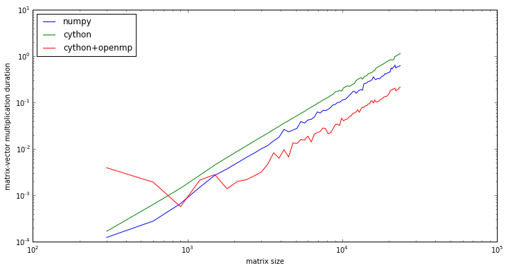
For large problem sizes the the cython+OpenMP implementation is faster than numpy.dot.
With this simple implementation, the speedup for large problem sizes is about:
((duration_ref / duration_cy_omp)[-10:]).mean()
3.0072232987815148
Obviously one could do a better job with more effort, since the theoretical limit of the speed-up is:
N_core
12
Further reading
OpenCL
OpenCL is an API for heterogenous computing, for example using GPUs for numerical computations. There is a python package called pyopencl that allows OpenCL code to be compiled, loaded and executed on the compute units completely from within Python. This is a nice way to work with OpenCL, because the time-consuming computations should be done on the compute units in compiled code, and in this Python only server as a control language.
%%file opencl-dense-mv.py

import pyopencl as cl
import numpy
import time

# problem size
n = 10000

# platform
platform_list = cl.get_platforms()
platform = platform_list[0]

# device
device_list = platform.get_devices()
device = device_list[0]

if False:
    print("Platform name:" + platform.name)
    print("Platform version:" + platform.version)
    print("Device name:" + device.name)
    print("Device type:" + cl.device_type.to_string(device.type))
    print("Device memory: " + str(device.global_mem_size//1024//1024) + ' MB')
    print("Device max clock speed:" + str(device.max_clock_frequency) + ' MHz')
    print("Device compute units:" + str(device.max_compute_units))

# context
ctx = cl.Context([device]) # or we can use cl.create_some_context()

# command queue
queue = cl.CommandQueue(ctx)

# kernel
KERNEL_CODE = """
//
// Matrix-vector multiplication: r = m * v
//
#define N %(mat_size)d
__kernel
void dmv_cl(__global float *m, __global float *v, __global float *r)
{
    int i, gid = get_global_id(0);

    r[gid] = 0;
    for (i = 0; i < N; i++)
    {
        r[gid] += m[gid * N + i] * v[i];
    }
}
"""

kernel_params = {"mat_size": n}
program = cl.Program(ctx, KERNEL_CODE % kernel_params).build()

# data
A = numpy.random.rand(n, n)
x = numpy.random.rand(n, 1)

# host buffers
h_y = numpy.empty(numpy.shape(x)).astype(numpy.float32)
h_A = numpy.real(A).astype(numpy.float32)
h_x = numpy.real(x).astype(numpy.float32)

# device buffers
mf = cl.mem_flags
d_A_buf = cl.Buffer(ctx, mf.READ_ONLY | mf.COPY_HOST_PTR, hostbuf=h_A)
d_x_buf = cl.Buffer(ctx, mf.READ_ONLY | mf.COPY_HOST_PTR, hostbuf=h_x)
d_y_buf = cl.Buffer(ctx, mf.WRITE_ONLY, size=h_y.nbytes)

# execute OpenCL code
t0 = time.time()
event = program.dmv_cl(queue, h_y.shape, None, d_A_buf, d_x_buf, d_y_buf)
event.wait()
cl.enqueue_copy(queue, h_y, d_y_buf)
t1 = time.time()

print "opencl elapsed time =", (t1-t0)

# Same calculation with numpy
t0 = time.time()
y = numpy.dot(h_A, h_x)
t1 = time.time()

print "numpy elapsed time =", (t1-t0)

# see if the results are the same
print "max deviation =", numpy.abs(y-h_y).max()
Overwriting opencl-dense-mv.py
!python opencl-dense-mv.py
/usr/local/lib/python2.7/dist-packages/pyopencl-2012.1-py2.7-linux-x86_64.egg/pyopencl/__init__.py:36: CompilerWarning: Non-empty compiler output encountered. Set the environment variable PYOPENCL_COMPILER_OUTPUT=1 to see more.
  "to see more.", CompilerWarning)
opencl elapsed time = 0.0188570022583
numpy elapsed time = 0.0755031108856
max deviation = 0.0136719
Further reading
Versions
%load_ext version_information

%version_information numpy, mpi4py, Cython