Jupyter Snippet NP ch12-code-listing
Jupyter Snippet NP ch12-code-listing
Chapter 12: Data processing and analysis with pandas
Robert Johansson
Source code listings for Numerical Python - Scientific Computing and Data Science Applications with Numpy, SciPy and Matplotlib (ISBN 978-1-484242-45-2).
%matplotlib inline
import matplotlib.pyplot as plt
import numpy as np
import pandas as pd
# pd.set_option('display.mpl_style', 'default')
import matplotlib as mpl
mpl.style.use('ggplot')
import seaborn as sns
Series object
s = pd.Series([909976, 8615246, 2872086, 2273305])
s
0     909976
1    8615246
2    2872086
3    2273305
dtype: int64
type(s)
pandas.core.series.Series
s.dtype
dtype('int64')
s.index
RangeIndex(start=0, stop=4, step=1)
s.values
array([ 909976, 8615246, 2872086, 2273305])
s.index = ["Stockholm", "London", "Rome", "Paris"]
s.name = "Population"
s
Stockholm     909976
London       8615246
Rome         2872086
Paris        2273305
Name: Population, dtype: int64
s = pd.Series([909976, 8615246, 2872086, 2273305],
              index=["Stockholm", "London", "Rome", "Paris"], name="Population")
s["London"]
8615246
s.Stockholm
909976
s[["Paris", "Rome"]]
Paris    2273305
Rome     2872086
Name: Population, dtype: int64
s.median(), s.mean(), s.std()
(2572695.5, 3667653.25, 3399048.5005155364)
s.min(), s.max()
(909976, 8615246)
s.quantile(q=0.25), s.quantile(q=0.5), s.quantile(q=0.75)
(1932472.75, 2572695.5, 4307876.0)
s.describe()
count    4.000000e+00
mean     3.667653e+06
std      3.399049e+06
min      9.099760e+05
25%      1.932473e+06
50%      2.572696e+06
75%      4.307876e+06
max      8.615246e+06
Name: Population, dtype: float64
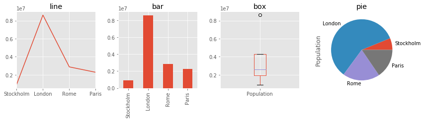
fig, axes = plt.subplots(1, 4, figsize=(12, 3.5))

s.plot(ax=axes[0], kind='line', title="line")
s.plot(ax=axes[1], kind='bar', title="bar")
s.plot(ax=axes[2], kind='box', title="box")
s.plot(ax=axes[3], kind='pie', title="pie")

fig.tight_layout()
fig.savefig("ch12-series-plot.pdf")
fig.savefig("ch12-series-plot.png")
DataFrame object
df = pd.DataFrame([[909976, 8615246, 2872086, 2273305],
                   ["Sweden", "United kingdom", "Italy", "France"]])
df
.dataframe tbody tr th {
    vertical-align: top;
}

.dataframe thead th {
    text-align: right;
}
df = pd.DataFrame([[909976, "Sweden"],
                   [8615246, "United kingdom"],
                   [2872086, "Italy"],
                   [2273305, "France"]])
df
.dataframe tbody tr th {
    vertical-align: top;
}

.dataframe thead th {
    text-align: right;
}
df.index = ["Stockholm", "London", "Rome", "Paris"]
df.columns = ["Population", "State"]
df
.dataframe tbody tr th {
    vertical-align: top;
}

.dataframe thead th {
    text-align: right;
}
df = pd.DataFrame([[909976, "Sweden"],
                   [8615246, "United kingdom"],
                   [2872086, "Italy"],
                   [2273305, "France"]],
                  index=["Stockholm", "London", "Rome", "Paris"],
                  columns=["Population", "State"])
df
.dataframe tbody tr th {
    vertical-align: top;
}

.dataframe thead th {
    text-align: right;
}
df = pd.DataFrame({"Population": [909976, 8615246, 2872086, 2273305],
                   "State": ["Sweden", "United kingdom", "Italy", "France"]},
                  index=["Stockholm", "London", "Rome", "Paris"])
df
.dataframe tbody tr th {
    vertical-align: top;
}

.dataframe thead th {
    text-align: right;
}
df.index
Index(['Stockholm', 'London', 'Rome', 'Paris'], dtype='object')
df.columns
Index(['Population', 'State'], dtype='object')
df.values
array([[909976, 'Sweden'],
       [8615246, 'United kingdom'],
       [2872086, 'Italy'],
       [2273305, 'France']], dtype=object)
df.Population
Stockholm     909976
London       8615246
Rome         2872086
Paris        2273305
Name: Population, dtype: int64
df["Population"]
Stockholm     909976
London       8615246
Rome         2872086
Paris        2273305
Name: Population, dtype: int64
type(df.Population)
pandas.core.series.Series
df.Population.Stockholm
909976
type(df.index)
pandas.core.indexes.base.Index
df.loc["Stockholm"]
Population    909976
State         Sweden
Name: Stockholm, dtype: object
type(df.loc["Stockholm"])
pandas.core.series.Series
df.loc[["Paris", "Rome"]]
.dataframe tbody tr th {
    vertical-align: top;
}

.dataframe thead th {
    text-align: right;
}
df.loc[["Paris", "Rome"], "Population"]
Paris    2273305
Rome     2872086
Name: Population, dtype: int64
df.loc["Paris", "Population"]
2273305
df.mean()
Population    3667653.25
dtype: float64
df.info()
<class 'pandas.core.frame.DataFrame'>
Index: 4 entries, Stockholm to Paris
Data columns (total 2 columns):
Population    4 non-null int64
State         4 non-null object
dtypes: int64(1), object(1)
memory usage: 256.0+ bytes
df.dtypes
Population     int64
State         object
dtype: object
df.head()
.dataframe tbody tr th {
    vertical-align: top;
}

.dataframe thead th {
    text-align: right;
}
!head -n5 /home/rob/datasets/european_cities.csv
Rank,City,State,Official population,Date of census/estimate
1,London[2], United Kingdom,"8,615,246",1 June 2014
2,Berlin, Germany,"3,437,916",31 May 2014
3,Madrid, Spain,"3,165,235",1 January 2014
4,Rome, Italy,"2,872,086",30 September 2014
Larger dataset
df_pop = pd.read_csv("european_cities.csv")
df_pop.head()
.dataframe tbody tr th {
    vertical-align: top;
}

.dataframe thead th {
    text-align: right;
}
df_pop = pd.read_csv("european_cities.csv", delimiter=",", encoding="utf-8", header=0)
df_pop.info()
<class 'pandas.core.frame.DataFrame'>
RangeIndex: 105 entries, 0 to 104
Data columns (total 5 columns):
Rank                       105 non-null int64
City                       105 non-null object
State                      105 non-null object
Population                 105 non-null object
Date of census/estimate    105 non-null object
dtypes: int64(1), object(4)
memory usage: 4.2+ KB
df_pop.head()
.dataframe tbody tr th {
    vertical-align: top;
}

.dataframe thead th {
    text-align: right;
}
df_pop["NumericPopulation"] = df_pop.Population.apply(lambda x: int(x.replace(",", "")))
df_pop["State"].values[:3]
array([' United Kingdom', ' Germany', ' Spain'], dtype=object)
df_pop["State"] = df_pop["State"].apply(lambda x: x.strip())
df_pop.head()
.dataframe tbody tr th {
    vertical-align: top;
}

.dataframe thead th {
    text-align: right;
}
df_pop.dtypes
Rank                        int64
City                       object
State                      object
Population                 object
Date of census/estimate    object
NumericPopulation           int64
dtype: object
df_pop2 = df_pop.set_index("City")
df_pop2 = df_pop2.sort_index()
df_pop2.head()
.dataframe tbody tr th {
    vertical-align: top;
}

.dataframe thead th {
    text-align: right;
}
df_pop2.head()
.dataframe tbody tr th {
    vertical-align: top;
}

.dataframe thead th {
    text-align: right;
}
df_pop3 = df_pop.set_index(["State", "City"]).sort_index(level=0)
df_pop3.head(7)
.dataframe tbody tr th {
    vertical-align: top;
}

.dataframe thead th {
    text-align: right;
}
df_pop3.loc["Sweden"]
.dataframe tbody tr th {
    vertical-align: top;
}

.dataframe thead th {
    text-align: right;
}
df_pop3.loc[("Sweden", "Gothenburg")]
Rank                                  53
Population                       528,014
Date of census/estimate    31 March 2013
NumericPopulation                 528014
Name: (Sweden, Gothenburg), dtype: object
df_pop.set_index("City").sort_values(["State", "NumericPopulation"], ascending=[False, True]).head()
.dataframe tbody tr th {
    vertical-align: top;
}

.dataframe thead th {
    text-align: right;
}
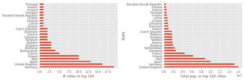
city_counts = df_pop.State.value_counts()
city_counts.name = "# cities in top 105"
df_pop3 = df_pop[["State", "City", "NumericPopulation"]].set_index(["State", "City"])
df_pop4 = df_pop3.sum(level="State").sort_values("NumericPopulation", ascending=False)
df_pop4.head()
.dataframe tbody tr th {
    vertical-align: top;
}

.dataframe thead th {
    text-align: right;
}
df_pop5 = (df_pop.drop("Rank", axis=1)
                 .groupby("State").sum()
                 .sort_values("NumericPopulation", ascending=False))
df_pop5.head()
.dataframe tbody tr th {
    vertical-align: top;
}

.dataframe thead th {
    text-align: right;
}
fig, (ax1, ax2) = plt.subplots(1, 2, figsize=(12, 4))

city_counts.plot(kind='barh', ax=ax1)
ax1.set_xlabel("# cities in top 105")
df_pop5.NumericPopulation.plot(kind='barh', ax=ax2)
ax2.set_xlabel("Total pop. in top 105 cities")

fig.tight_layout()
fig.savefig("ch12-state-city-counts-sum.pdf")
Time series
Basics
import datetime
pd.date_range("2015-1-1", periods=31)
DatetimeIndex(['2015-01-01', '2015-01-02', '2015-01-03', '2015-01-04',
               '2015-01-05', '2015-01-06', '2015-01-07', '2015-01-08',
               '2015-01-09', '2015-01-10', '2015-01-11', '2015-01-12',
               '2015-01-13', '2015-01-14', '2015-01-15', '2015-01-16',
               '2015-01-17', '2015-01-18', '2015-01-19', '2015-01-20',
               '2015-01-21', '2015-01-22', '2015-01-23', '2015-01-24',
               '2015-01-25', '2015-01-26', '2015-01-27', '2015-01-28',
               '2015-01-29', '2015-01-30', '2015-01-31'],
              dtype='datetime64[ns]', freq='D')
pd.date_range(datetime.datetime(2015, 1, 1), periods=31)
DatetimeIndex(['2015-01-01', '2015-01-02', '2015-01-03', '2015-01-04',
               '2015-01-05', '2015-01-06', '2015-01-07', '2015-01-08',
               '2015-01-09', '2015-01-10', '2015-01-11', '2015-01-12',
               '2015-01-13', '2015-01-14', '2015-01-15', '2015-01-16',
               '2015-01-17', '2015-01-18', '2015-01-19', '2015-01-20',
               '2015-01-21', '2015-01-22', '2015-01-23', '2015-01-24',
               '2015-01-25', '2015-01-26', '2015-01-27', '2015-01-28',
               '2015-01-29', '2015-01-30', '2015-01-31'],
              dtype='datetime64[ns]', freq='D')
pd.date_range("2015-1-1 00:00", "2015-1-1 12:00", freq="H")
DatetimeIndex(['2015-01-01 00:00:00', '2015-01-01 01:00:00',
               '2015-01-01 02:00:00', '2015-01-01 03:00:00',
               '2015-01-01 04:00:00', '2015-01-01 05:00:00',
               '2015-01-01 06:00:00', '2015-01-01 07:00:00',
               '2015-01-01 08:00:00', '2015-01-01 09:00:00',
               '2015-01-01 10:00:00', '2015-01-01 11:00:00',
               '2015-01-01 12:00:00'],
              dtype='datetime64[ns]', freq='H')
ts1 = pd.Series(np.arange(31), index=pd.date_range("2015-1-1", periods=31))
ts1.head()
2015-01-01    0
2015-01-02    1
2015-01-03    2
2015-01-04    3
2015-01-05    4
Freq: D, dtype: int64
ts1["2015-1-3"]
2
ts1.index[2]
Timestamp('2015-01-03 00:00:00', freq='D')
ts1.index[2].year, ts1.index[2].month, ts1.index[2].day
(2015, 1, 3)
ts1.index[2].nanosecond
0
ts1.index[2].to_pydatetime()
datetime.datetime(2015, 1, 3, 0, 0)
ts2 = pd.Series(np.random.rand(2),
                index=[datetime.datetime(2015, 1, 1), datetime.datetime(2015, 2, 1)])
ts2
2015-01-01    0.431883
2015-02-01    0.794106
dtype: float64
periods = pd.PeriodIndex([pd.Period('2015-01'), pd.Period('2015-02'), pd.Period('2015-03')])
ts3 = pd.Series(np.random.rand(3), periods)
ts3
2015-01    0.102122
2015-02    0.952019
2015-03    0.874310
Freq: M, dtype: float64
ts3.index
PeriodIndex(['2015-01', '2015-02', '2015-03'], dtype='period[M]', freq='M')
ts2.to_period('M')
2015-01    0.431883
2015-02    0.794106
Freq: M, dtype: float64
pd.date_range("2015-1-1", periods=12, freq="M").to_period()
PeriodIndex(['2015-01', '2015-02', '2015-03', '2015-04', '2015-05', '2015-06',
             '2015-07', '2015-08', '2015-09', '2015-10', '2015-11', '2015-12'],
            dtype='period[M]', freq='M')
Temperature time series example
!head -n 5 temperature_outdoor_2014.tsv
1388530986	4.380000
1388531586	4.250000
1388532187	4.190000
1388532787	4.060000
1388533388	4.060000
df1 = pd.read_csv('temperature_outdoor_2014.tsv', delimiter="\t", names=["time", "outdoor"])
df2 = pd.read_csv('temperature_indoor_2014.tsv', delimiter="\t", names=["time", "indoor"])
df1.head()
.dataframe tbody tr th {
    vertical-align: top;
}

.dataframe thead th {
    text-align: right;
}
df2.head()
.dataframe tbody tr th {
    vertical-align: top;
}

.dataframe thead th {
    text-align: right;
}
df1.time = (pd.to_datetime(df1.time.values, unit="s")
              .tz_localize('UTC').tz_convert('Europe/Stockholm'))
df1 = df1.set_index("time")
df2.time = (pd.to_datetime(df2.time.values, unit="s")
              .tz_localize('UTC').tz_convert('Europe/Stockholm'))
df2 = df2.set_index("time")
df1.head()
.dataframe tbody tr th {
    vertical-align: top;
}

.dataframe thead th {
    text-align: right;
}
df1.index[0]
Timestamp('2014-01-01 00:03:06+0100', tz='Europe/Stockholm')
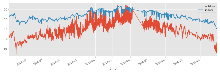
fig, ax = plt.subplots(1, 1, figsize=(12, 4))
df1.plot(ax=ax)
df2.plot(ax=ax)

fig.tight_layout()
fig.savefig("ch12-timeseries-temperature-2014.pdf")
# select january data
df1.info()
<class 'pandas.core.frame.DataFrame'>
DatetimeIndex: 49548 entries, 2014-01-01 00:03:06+01:00 to 2014-12-30 23:56:35+01:00
Data columns (total 1 columns):
outdoor    49548 non-null float64
dtypes: float64(1)
memory usage: 774.2 KB
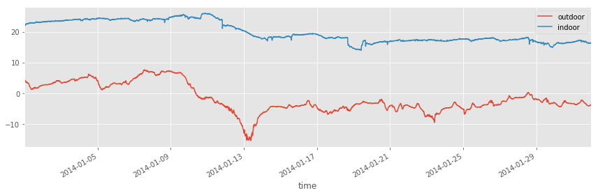
df1_jan = df1[(df1.index > "2014-1-1") & (df1.index < "2014-2-1")]
df1.index < "2014-2-1"
array([ True, True, True, ..., False, False, False])
df1_jan.info()
<class 'pandas.core.frame.DataFrame'>
DatetimeIndex: 4452 entries, 2014-01-01 00:03:06+01:00 to 2014-01-31 23:56:58+01:00
Data columns (total 1 columns):
outdoor    4452 non-null float64
dtypes: float64(1)
memory usage: 69.6 KB
df2_jan = df2["2014-1-1":"2014-1-31"]
fig, ax = plt.subplots(1, 1, figsize=(12, 4))

df1_jan.plot(ax=ax)
df2_jan.plot(ax=ax)

fig.tight_layout()
fig.savefig("ch12-timeseries-selected-month.pdf")
# group by month
df1_month = df1.reset_index()
df1_month["month"] = df1_month.time.apply(lambda x: x.month)
df1_month.head()
.dataframe tbody tr th {
    vertical-align: top;
}

.dataframe thead th {
    text-align: right;
}
df1_month = df1_month.groupby("month").aggregate(np.mean)
df2_month = df2.reset_index()
df2_month["month"] = df2_month.time.apply(lambda x: x.month)
df2_month = df2_month.groupby("month").aggregate(np.mean)
df_month = df1_month.join(df2_month)
df_month.head(3)
.dataframe tbody tr th {
    vertical-align: top;
}

.dataframe thead th {
    text-align: right;
}
df_month = pd.concat([df.to_period("M").groupby(level=0).mean() for df in [df1, df2]], axis=1)
/Users/rob/miniconda3/envs/py3.6/lib/python3.6/site-packages/pandas/core/arrays/datetimes.py:1172: UserWarning: Converting to PeriodArray/Index representation will drop timezone information.
  "will drop timezone information.", UserWarning)
/Users/rob/miniconda3/envs/py3.6/lib/python3.6/site-packages/pandas/core/arrays/datetimes.py:1172: UserWarning: Converting to PeriodArray/Index representation will drop timezone information.
  "will drop timezone information.", UserWarning)
df_month.head(3)
.dataframe tbody tr th {
    vertical-align: top;
}

.dataframe thead th {
    text-align: right;
}
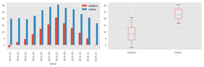
fig, axes = plt.subplots(1, 2, figsize=(12, 4))

df_month.plot(kind='bar', ax=axes[0])
df_month.plot(kind='box', ax=axes[1])

fig.tight_layout()
fig.savefig("ch12-grouped-by-month.pdf")
df_month
.dataframe tbody tr th {
    vertical-align: top;
}

.dataframe thead th {
    text-align: right;
}
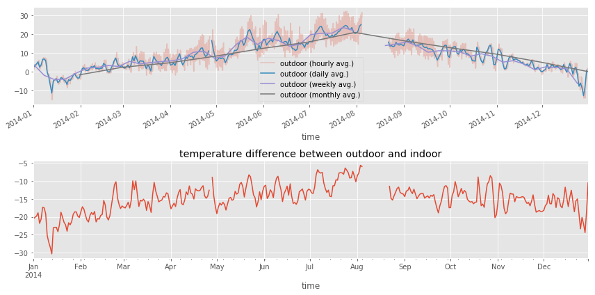
# resampling
df1_hour = df1.resample("H").mean()
df1_hour.columns = ["outdoor (hourly avg.)"]
df1_day = df1.resample("D").mean()
df1_day.columns = ["outdoor (daily avg.)"]
df1_week = df1.resample("7D").mean()
df1_week.columns = ["outdoor (weekly avg.)"]
df1_month = df1.resample("M").mean()
df1_month.columns = ["outdoor (monthly avg.)"]
df_diff = (df1.resample("D").mean().outdoor - df2.resample("D").mean().indoor)
fig, (ax1, ax2) = plt.subplots(2, 1, figsize=(12, 6))

df1_hour.plot(ax=ax1, alpha=0.25)
df1_day.plot(ax=ax1)
df1_week.plot(ax=ax1)
df1_month.plot(ax=ax1)

df_diff.plot(ax=ax2)
ax2.set_title("temperature difference between outdoor and indoor")

fig.tight_layout()
fig.savefig("ch12-timeseries-resampled.pdf")
/Users/rob/miniconda3/envs/py3.6/lib/python3.6/site-packages/pandas/core/arrays/datetimes.py:1172: UserWarning: Converting to PeriodArray/Index representation will drop timezone information.
  "will drop timezone information.", UserWarning)
pd.concat([df1.resample("5min").mean().rename(columns={"outdoor": 'None'}),
           df1.resample("5min").ffill().rename(columns={"outdoor": 'ffill'}),
           df1.resample("5min").bfill().rename(columns={"outdoor": 'bfill'})], axis=1).head()
.dataframe tbody tr th {
    vertical-align: top;
}

.dataframe thead th {
    text-align: right;
}
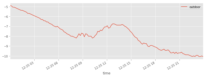
Selected day
df1_dec25 = df1[(df1.index < "2014-9-1") & (df1.index >= "2014-8-1")].resample("D")
df1_dec25 = df1.loc["2014-12-25"]
df1_dec25.head(5)
.dataframe tbody tr th {
    vertical-align: top;
}

.dataframe thead th {
    text-align: right;
}
df2_dec25 = df2.loc["2014-12-25"]
df2_dec25.head(5)
.dataframe tbody tr th {
    vertical-align: top;
}

.dataframe thead th {
    text-align: right;
}
df1_dec25.describe().T
.dataframe tbody tr th {
    vertical-align: top;
}

.dataframe thead th {
    text-align: right;
}
fig, ax = plt.subplots(1, 1, figsize=(12, 4))

df1_dec25.plot(ax=ax)

fig.savefig("ch12-timeseries-selected-month.pdf")
df1.index
DatetimeIndex(['2014-01-01 00:03:06+01:00', '2014-01-01 00:13:06+01:00',
               '2014-01-01 00:23:07+01:00', '2014-01-01 00:33:07+01:00',
               '2014-01-01 00:43:08+01:00', '2014-01-01 00:53:08+01:00',
               '2014-01-01 01:03:09+01:00', '2014-01-01 01:13:09+01:00',
               '2014-01-01 01:23:10+01:00', '2014-01-01 01:33:26+01:00',
               ...
               '2014-12-30 22:26:30+01:00', '2014-12-30 22:36:31+01:00',
               '2014-12-30 22:46:31+01:00', '2014-12-30 22:56:32+01:00',
               '2014-12-30 23:06:32+01:00', '2014-12-30 23:16:33+01:00',
               '2014-12-30 23:26:33+01:00', '2014-12-30 23:36:34+01:00',
               '2014-12-30 23:46:35+01:00', '2014-12-30 23:56:35+01:00'],
              dtype='datetime64[ns, Europe/Stockholm]', name='time', length=49548, freq=None)
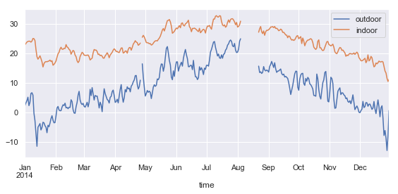
Seaborn statistical visualization library
sns.set(style="darkgrid")
#sns.set(style="whitegrid")
df1 = pd.read_csv('temperature_outdoor_2014.tsv', delimiter="\t", names=["time", "outdoor"])
df1.time = pd.to_datetime(df1.time.values, unit="s").tz_localize('UTC').tz_convert('Europe/Stockholm')

df1 = df1.set_index("time").resample("10min").mean()
df2 = pd.read_csv('temperature_indoor_2014.tsv', delimiter="\t", names=["time", "indoor"])
df2.time = pd.to_datetime(df2.time.values, unit="s").tz_localize('UTC').tz_convert('Europe/Stockholm')
df2 = df2.set_index("time").resample("10min").mean()
df_temp = pd.concat([df1, df2], axis=1)
fig, ax = plt.subplots(1, 1, figsize=(8, 4))
df_temp.resample("D").mean().plot(y=["outdoor", "indoor"], ax=ax)
fig.tight_layout()
fig.savefig("ch12-seaborn-plot.pdf")
/Users/rob/miniconda3/envs/py3.6/lib/python3.6/site-packages/pandas/core/arrays/datetimes.py:1172: UserWarning: Converting to PeriodArray/Index representation will drop timezone information.
  "will drop timezone information.", UserWarning)
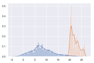
#sns.kdeplot(df_temp["outdoor"].dropna().values, shade=True, cumulative=True);
sns.distplot(df_temp.to_period("M")["outdoor"]["2014-04"].dropna().values, bins=50);
sns.distplot(df_temp.to_period("M")["indoor"]["2014-04"].dropna().values, bins=50);

plt.savefig("ch12-seaborn-distplot.pdf")
/Users/rob/miniconda3/envs/py3.6/lib/python3.6/site-packages/pandas/core/arrays/datetimes.py:1172: UserWarning: Converting to PeriodArray/Index representation will drop timezone information.
  "will drop timezone information.", UserWarning)
/Users/rob/miniconda3/envs/py3.6/lib/python3.6/site-packages/pandas/core/arrays/datetimes.py:1172: UserWarning: Converting to PeriodArray/Index representation will drop timezone information.
  "will drop timezone information.", UserWarning)
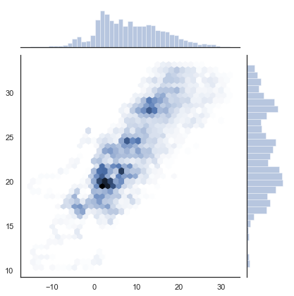
with sns.axes_style("white"):
    sns.jointplot(df_temp.resample("H").mean()["outdoor"].values,
                  df_temp.resample("H").mean()["indoor"].values, kind="hex");

plt.savefig("ch12-seaborn-jointplot.pdf")
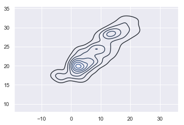
sns.kdeplot(df_temp.resample("H").mean()["outdoor"].dropna().values,
            df_temp.resample("H").mean()["indoor"].dropna().values, shade=False);

plt.savefig("ch12-seaborn-kdeplot.pdf")
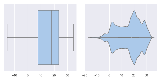
fig, (ax1, ax2) = plt.subplots(1, 2, figsize=(8, 4))

sns.boxplot(df_temp.dropna(), ax=ax1, palette="pastel")
sns.violinplot(df_temp.dropna(), ax=ax2, palette="pastel")

fig.tight_layout()
fig.savefig("ch12-seaborn-boxplot-violinplot.pdf")
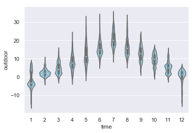
sns.violinplot(x=df_temp.dropna().index.month, y=df_temp.dropna().outdoor, color="skyblue");

plt.savefig("ch12-seaborn-violinplot.pdf")
df_temp["month"] = df_temp.index.month
df_temp["hour"] = df_temp.index.hour
df_temp.head()
.dataframe tbody tr th {
    vertical-align: top;
}

.dataframe thead th {
    text-align: right;
}
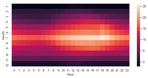
table = pd.pivot_table(df_temp, values='outdoor', index=['month'], columns=['hour'], aggfunc=np.mean)
table
.dataframe tbody tr th {
    vertical-align: top;
}

.dataframe thead th {
    text-align: right;
}
fig, ax = plt.subplots(1, 1, figsize=(8, 4))
sns.heatmap(table, ax=ax);

fig.tight_layout()
fig.savefig("ch12-seaborn-heatmap.pdf")
Versions
%reload_ext version_information
%version_information numpy, matplotlib, pandas, seaborn