Jupyter Snippet NP ch09-code-listing
Jupyter Snippet NP ch09-code-listing
Chapter 9: Ordinary differential equations
Robert Johansson
Source code listings for Numerical Python - Scientific Computing and Data Science Applications with Numpy, SciPy and Matplotlib (ISBN 978-1-484242-45-2).
import numpy as np
%matplotlib inline
%config InlineBackend.figure_format='retina'
import matplotlib.pyplot as plt
import matplotlib as mpl
# mpl.rcParams['text.usetex'] = True
mpl.rcParams['mathtext.fontset'] = 'stix'
mpl.rcParams['font.family'] = 'serif'
mpl.rcParams['font.sans-serif'] = 'stix'
import sympy
sympy.init_printing()
from scipy import integrate
Symbolic ODE solving with SymPy
Newton’s law of cooling
t, k, T0, Ta = sympy.symbols("t, k, T_0, T_a")
T = sympy.Function("T")
ode = T(t).diff(t) + k*(T(t) - Ta)
ode
$\displaystyle k \left(- T_{a} + T{\left(t \right)}\right) + \frac{d}{d t} T{\left(t \right)}$
ode_sol = sympy.dsolve(ode)
ode_sol
$\displaystyle T{\left(t \right)} = C_{1} e^{- k t} + T_{a}$
ode_sol.lhs
$\displaystyle T{\left(t \right)}$
ode_sol.rhs
$\displaystyle C_{1} e^{- k t} + T_{a}$
ics = {T(0): T0}
ics
$\displaystyle \left{ T{\left(0 \right)} : T_{0}\right}$
C_eq = ode_sol.subs(t, 0).subs(ics)
C_eq
$\displaystyle T_{0} = C_{1} + T_{a}$
C_sol = sympy.solve(C_eq)
C_sol
$\displaystyle \left[ \left{ C_{1} : T_{0} - T_{a}\right}\right]$
ode_sol.subs(C_sol[0])
$\displaystyle T{\left(t \right)} = T_{a} + \left(T_{0} - T_{a}\right) e^{- k t}$
Function for applying initial conditions
def apply_ics(sol, ics, x, known_params):
    """
    Apply the initial conditions (ics), given as a dictionary on
    the form ics = {y(0): y0: y(x).diff(x).subs(x, 0): yp0, ...}
    to the solution of the ODE with indepdendent variable x.
    The undetermined integration constants C1, C2, ... are extracted
    from the free symbols of the ODE solution, excluding symbols in
    the known_params list.
    """
    free_params = sol.free_symbols - set(known_params)
    eqs = [(sol.lhs.diff(x, n) - sol.rhs.diff(x, n)).subs(x, 0).subs(ics)
           for n in range(len(ics))]
    sol_params = sympy.solve(eqs, free_params)
    return sol.subs(sol_params)
ode_sol
$\displaystyle T{\left(t \right)} = C_{1} e^{- k t} + T_{a}$
apply_ics(ode_sol, ics, t, [k, Ta])
$\displaystyle T{\left(t \right)} = T_{a} + \left(T_{0} - T_{a}\right) e^{- k t}$
ode_sol = apply_ics(ode_sol, ics, t, [k, Ta]).simplify()
ode_sol
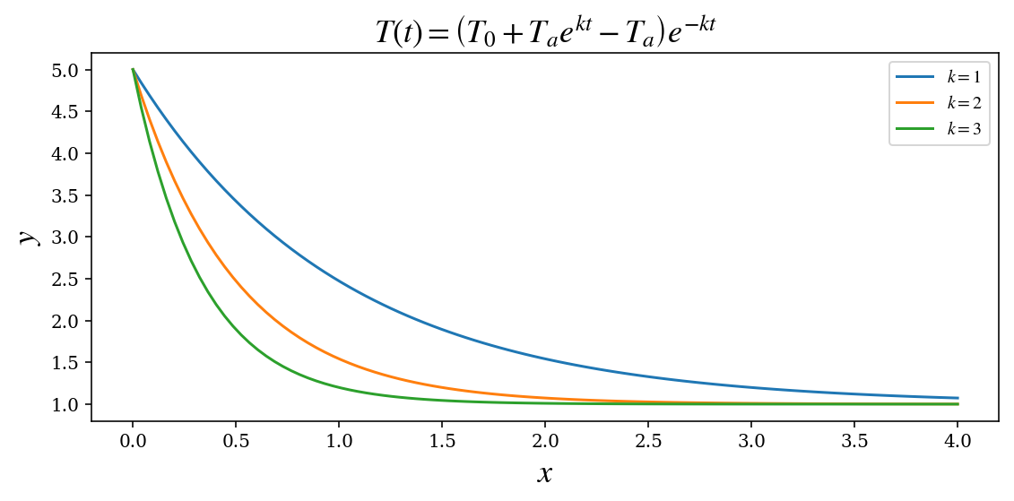
$\displaystyle T{\left(t \right)} = \left(T_{0} + T_{a} e^{k t} - T_{a}\right) e^{- k t}$
y_x = sympy.lambdify((t, k), ode_sol.rhs.subs({T0: 5, Ta: 1}), 'numpy')
fig, ax = plt.subplots(figsize=(8, 4))

x = np.linspace(0, 4, 100)

for k in [1, 2, 3]:
    ax.plot(x, y_x(x, k), label=r"$k=%d$" % k)

ax.set_title(r"$%s$" % sympy.latex(ode_sol), fontsize=18)
ax.set_xlabel(r"$x$", fontsize=18)
ax.set_ylabel(r"$y$", fontsize=18)
ax.legend()

fig.tight_layout()
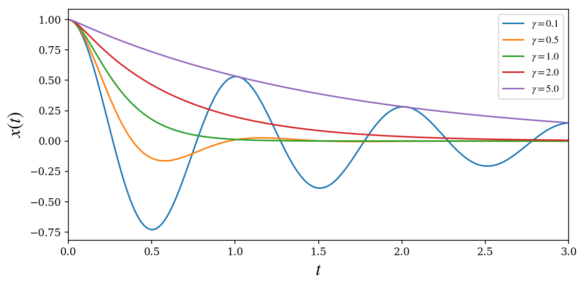
Damped harmonic oscillator
t, omega0 = sympy.symbols("t, omega_0", positive=True)
gamma = sympy.symbols("gamma", complex=True)
x = sympy.Function("x")
ode = x(t).diff(t, 2) + 2 * gamma * omega0 * x(t).diff(t) + omega0**2 * x(t)
ode
$\displaystyle 2 \gamma \omega_{0} \frac{d}{d t} x{\left(t \right)} + \omega_{0}^{2} x{\left(t \right)} + \frac{d^{2}}{d t^{2}} x{\left(t \right)}$
ode_sol = sympy.dsolve(ode)
ode_sol
$\displaystyle x{\left(t \right)} = C_{1} e^{\omega_{0} t \left(- \gamma - \sqrt{\gamma^{2} - 1}\right)} + C_{2} e^{\omega_{0} t \left(- \gamma + \sqrt{\gamma^{2} - 1}\right)}$
ics = {x(0): 1, x(t).diff(t).subs(t, 0): 0}
ics
$\displaystyle \left{ x{\left(0 \right)} : 1, \ \left. \frac{d}{d t} x{\left(t \right)} \right|_{\substack{ t=0 }} : 0\right}$
x_t_sol = apply_ics(ode_sol, ics, t, [omega0, gamma])
x_t_sol
$\displaystyle x{\left(t \right)} = \left(- \frac{\gamma}{2 \sqrt{\gamma^{2} - 1}} + \frac{1}{2}\right) e^{\omega_{0} t \left(- \gamma - \sqrt{\gamma^{2} - 1}\right)} + \left(\frac{\gamma}{2 \sqrt{\gamma^{2} - 1}} + \frac{1}{2}\right) e^{\omega_{0} t \left(- \gamma + \sqrt{\gamma^{2} - 1}\right)}$
x_t_critical = sympy.limit(x_t_sol.rhs, gamma, 1)
x_t_critical
$\displaystyle \left(\omega_{0} t + 1\right) e^{- \omega_{0} t}$
fig, ax = plt.subplots(figsize=(8, 4))

tt = np.linspace(0, 3, 250)
for g in [0.1, 0.5, 1, 2.0, 5.0]:
    if g == 1:
        x_t = sympy.lambdify(t, x_t_critical.subs({omega0: 2.0 * sympy.pi}), 'numpy')
    else:
        x_t = sympy.lambdify(t, x_t_sol.rhs.subs({omega0: 2.0 * sympy.pi, gamma: g}), 'numpy')
    ax.plot(tt, x_t(tt).real, label=r"$\gamma = %.1f$" % g)

ax.set_xlabel(r"$t$", fontsize=18)
ax.set_ylabel(r"$x(t)$", fontsize=18)
ax.set_xlim(0, 3)
ax.legend()

fig.tight_layout()
fig.savefig('ch9-harmonic-oscillator.pdf')
# example of equation that sympy cannot solve
x = sympy.symbols("x")
y = sympy.Function("y")
f = y(x)**2 + x
sympy.Eq(y(x).diff(x, x), f)
$\displaystyle \frac{d^{2}}{d x^{2}} y{\left(x \right)} = x + y^{2}{\left(x \right)}$
# sympy is unable to solve this differential equation
sympy.dsolve(y(x).diff(x, x) - f)
---------------------------------------------------------------------------

NotImplementedError                       Traceback (most recent call last)

<ipython-input-45-811796dbc135> in <module>
      1 # sympy is unable to solve this differential equation
----> 2 sympy.dsolve(y(x).diff(x, x) - f)


~/miniconda3/envs/py3.6/lib/python3.6/site-packages/sympy/solvers/ode.py in dsolve(eq, func, hint, simplify, ics, xi, eta, x0, n, **kwargs)
    639         hints = _desolve(eq, func=func,
    640             hint=hint, simplify=True, xi=xi, eta=eta, type='ode', ics=ics,
--> 641             x0=x0, n=n, **kwargs)
    642
    643         eq = hints.pop('eq', eq)


~/miniconda3/envs/py3.6/lib/python3.6/site-packages/sympy/solvers/deutils.py in _desolve(eq, func, hint, ics, simplify, **kwargs)
    233             raise ValueError(string + str(eq) + " does not match hint " + hint)
    234         else:
--> 235             raise NotImplementedError(dummy + "solve" + ": Cannot solve " + str(eq))
    236     if hint == 'default':
    237         return _desolve(eq, func, ics=ics, hint=hints['default'], simplify=simplify,


NotImplementedError: solve: Cannot solve -x - y(x)**2 + Derivative(y(x), (x, 2))
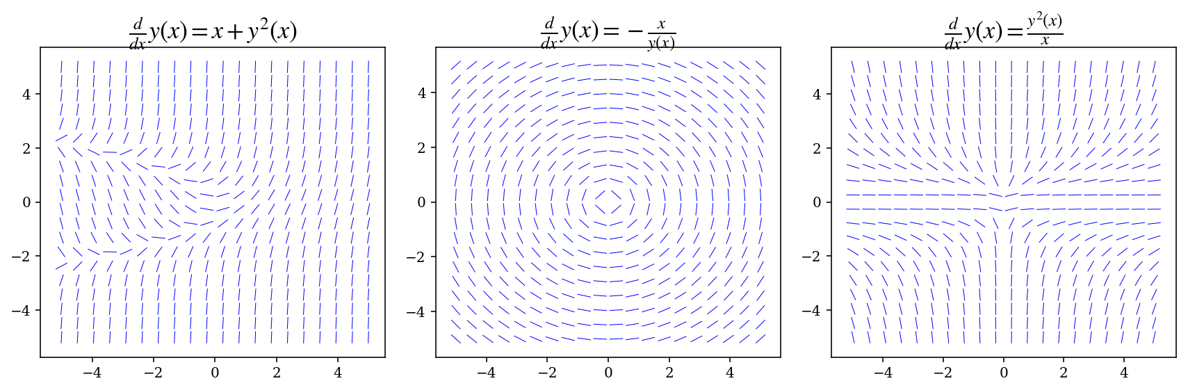
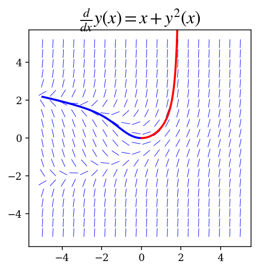
Direction fields
def  plot_direction_field(x, y_x, f_xy, x_lim=(-5, 5), y_lim=(-5, 5), ax=None):

    f_np = sympy.lambdify((x, y_x), f_xy, 'numpy')

    x_vec = np.linspace(x_lim[0], x_lim[1], 20)
    y_vec = np.linspace(y_lim[0], y_lim[1], 20)

    if ax is None:
        _, ax = plt.subplots(figsize=(4, 4))

    dx = x_vec[1] - x_vec[0]
    dy = y_vec[1] - y_vec[0]

    for m, xx in enumerate(x_vec):
        for n, yy in enumerate(y_vec):
            Dy = f_np(xx, yy) * dx
            Dx = 0.8 * dx**2 / np.sqrt(dx**2 + Dy**2)
            Dy = 0.8 * Dy*dy / np.sqrt(dx**2 + Dy**2)
            ax.plot([xx - Dx/2, xx + Dx/2],
                    [yy - Dy/2, yy + Dy/2], 'b', lw=0.5)
    ax.axis('tight')

    ax.set_title(r"$%s$" %
                 (sympy.latex(sympy.Eq(y(x).diff(x), f_xy))),
                 fontsize=18)

    return ax
x = sympy.symbols("x")
y = sympy.Function("y")
fig, axes = plt.subplots(1, 3, figsize=(12, 4))

plot_direction_field(x, y(x), y(x)**2 + x, ax=axes[0])
plot_direction_field(x, y(x), -x / y(x), ax=axes[1])
plot_direction_field(x, y(x), y(x)**2 / x, ax=axes[2])

fig.tight_layout()
fig.savefig('ch9-direction-field.pdf')
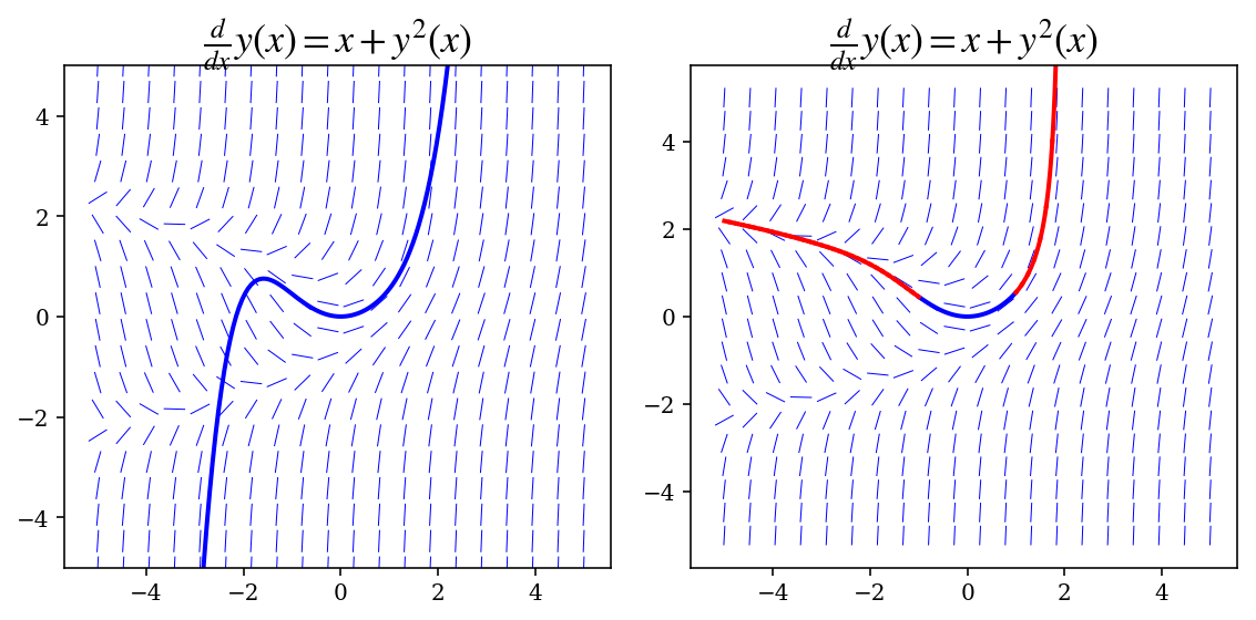
Inexact solutions to ODEs
x = sympy.symbols("x")
y = sympy.Function("y")
f = y(x)**2 + x
#f = sympy.cos(y(x)**2) + x
#f = sympy.sqrt(y(x)) * sympy.cos(x**2)
#f = y(x)**2 / x
sympy.Eq(y(x).diff(x), f)
$\displaystyle \frac{d}{d x} y{\left(x \right)} = x + y^{2}{\left(x \right)}$
ics = {y(0): 0}
ode_sol = sympy.dsolve(y(x).diff(x) - f)
ode_sol
$\displaystyle y{\left(x \right)} = \frac{x^{2} \left(2 C_{1}^{3} + 1\right)}{2} + \frac{x^{5} \left(10 C_{1}^{3} \left(6 C_{1}^{3} + 1\right) + 20 C_{1}^{3} + 3\right)}{60} + C_{1} + \frac{C_{1} x^{3} \left(3 C_{1}^{3} + 1\right)}{3} + C_{1}^{2} x + \frac{C_{1}^{2} x^{4} \left(12 C_{1}^{3} + 5\right)}{12} + O\left(x^{6}\right)$
ode_sol = apply_ics(ode_sol, {y(0): 0}, x, [])
ode_sol
$\displaystyle y{\left(x \right)} = \frac{x^{2}}{2} + \frac{x^{5}}{20} + O\left(x^{6}\right)$
ode_sol = sympy.dsolve(y(x).diff(x) - f, ics=ics)
ode_sol
$\displaystyle y{\left(x \right)} = \frac{x^{2}}{2} + \frac{x^{5}}{20} + O\left(x^{6}\right)$
fig, axes = plt.subplots(1, 2, figsize=(8, 4))

plot_direction_field(x, y(x), f, ax=axes[0])
x_vec = np.linspace(-3, 3, 100)
axes[0].plot(x_vec, sympy.lambdify(x, ode_sol.rhs.removeO())(x_vec), 'b', lw=2)
axes[0].set_ylim(-5, 5)

plot_direction_field(x, y(x), f, ax=axes[1])
x_vec = np.linspace(-1, 1, 100)
axes[1].plot(x_vec, sympy.lambdify(x, ode_sol.rhs.removeO())(x_vec), 'b', lw=2)

ode_sol_m = ode_sol_p = ode_sol
dx = 0.125
for x0 in np.arange(1, 2., dx):
    x_vec = np.linspace(x0, x0 + dx, 100)
    ics = {y(x0): ode_sol_p.rhs.removeO().subs(x, x0)}
    ode_sol_p = sympy.dsolve(y(x).diff(x) - f, ics=ics, n=6)
    axes[1].plot(x_vec, sympy.lambdify(x, ode_sol_p.rhs.removeO())(x_vec), 'r', lw=2)

for x0 in np.arange(-1, -5, -dx):
    x_vec = np.linspace(x0, x0 - dx, 100)
    ics = {y(x0): ode_sol_m.rhs.removeO().subs(x, x0)}
    ode_sol_m = sympy.dsolve(y(x).diff(x) - f, ics=ics, n=6)
    axes[1].plot(x_vec, sympy.lambdify(x, ode_sol_m.rhs.removeO())(x_vec), 'r', lw=2)

fig.tight_layout()
fig.savefig("ch9-direction-field-and-approx-sol.pdf")
Laplace transformation method
t = sympy.symbols("t", positive=True)
s, Y = sympy.symbols("s, Y", real=True)
y = sympy.Function("y")
ode = y(t).diff(t, 2) + 2 * y(t).diff(t) + 10 * y(t) - 2 * sympy.sin(3*t)
ode
$\displaystyle 10 y{\left(t \right)} - 2 \sin{\left(3 t \right)} + 2 \frac{d}{d t} y{\left(t \right)} + \frac{d^{2}}{d t^{2}} y{\left(t \right)}$
L_y = sympy.laplace_transform(y(t), t, s)
L_y
$\displaystyle \mathcal{L}_{t}\left[y{\left(t \right)}\right]\left(s\right)$
L_ode = sympy.laplace_transform(ode, t, s, noconds=True)
L_ode
$\displaystyle 10 \mathcal{L}{t}\left[y{\left(t \right)}\right]\left(s\right) + 2 \mathcal{L}{t}\left[\frac{d}{d t} y{\left(t \right)}\right]\left(s\right) + \mathcal{L}_{t}\left[\frac{d^{2}}{d t^{2}} y{\left(t \right)}\right]\left(s\right) - \frac{6}{s^{2} + 9}$
def laplace_transform_derivatives(e):
    """
    Evaluate the laplace transforms of derivatives of functions
    """
    if isinstance(e, sympy.LaplaceTransform):
        if isinstance(e.args[0], sympy.Derivative):
            d, t, s = e.args
            n = d.args[1][1]
            return ((s**n) * sympy.LaplaceTransform(d.args[0], t, s) -
                    sum([s**(n-i) * sympy.diff(d.args[0], t, i-1).subs(t, 0)
                         for i in range(1, n+1)]))

    if isinstance(e, (sympy.Add, sympy.Mul)):
        t = type(e)
        return t(*[laplace_transform_derivatives(arg) for arg in e.args])

    return e
L_ode
$\displaystyle 10 \mathcal{L}{t}\left[y{\left(t \right)}\right]\left(s\right) + 2 \mathcal{L}{t}\left[\frac{d}{d t} y{\left(t \right)}\right]\left(s\right) + \mathcal{L}_{t}\left[\frac{d^{2}}{d t^{2}} y{\left(t \right)}\right]\left(s\right) - \frac{6}{s^{2} + 9}$
L_ode_2 = laplace_transform_derivatives(L_ode)
L_ode_2
$\displaystyle s^{2} \mathcal{L}{t}\left[y{\left(t \right)}\right]\left(s\right) + 2 s \mathcal{L}{t}\left[y{\left(t \right)}\right]\left(s\right) - s y{\left(0 \right)} + 10 \mathcal{L}{t}\left[y{\left(t \right)}\right]\left(s\right) - 2 y{\left(0 \right)} - \left. \frac{d}{d t} y{\left(t \right)} \right|{\substack{ t=0 }} - \frac{6}{s^{2} + 9}$
L_ode_3 = L_ode_2.subs(L_y, Y)
L_ode_3
$\displaystyle Y s^{2} + 2 Y s + 10 Y - s y{\left(0 \right)} - 2 y{\left(0 \right)} - \left. \frac{d}{d t} y{\left(t \right)} \right|_{\substack{ t=0 }} - \frac{6}{s^{2} + 9}$
ics = {y(0): 1, y(t).diff(t).subs(t, 0): 0}
ics
$\displaystyle \left{ y{\left(0 \right)} : 1, \ \left. \frac{d}{d t} y{\left(t \right)} \right|_{\substack{ t=0 }} : 0\right}$
L_ode_4 = L_ode_3.subs(ics)
L_ode_4
$\displaystyle Y s^{2} + 2 Y s + 10 Y - s - 2 - \frac{6}{s^{2} + 9}$
Y_sol = sympy.solve(L_ode_4, Y)
Y_sol
$\displaystyle \left[ \frac{s^{3} + 2 s^{2} + 9 s + 24}{s^{4} + 2 s^{3} + 19 s^{2} + 18 s + 90}\right]$
sympy.apart(Y_sol[0])
$\displaystyle - \frac{6 \left(2 s - 1\right)}{37 \left(s^{2} + 9\right)} + \frac{49 s + 92}{37 \left(s^{2} + 2 s + 10\right)}$
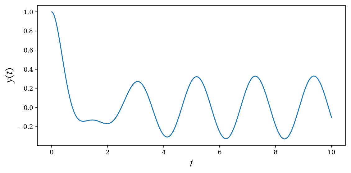
y_sol = sympy.inverse_laplace_transform(Y_sol[0], s, t)
sympy.simplify(y_sol)
$\displaystyle \frac{\left(6 e^{t} \sin{\left(3 t \right)} - 36 e^{t} \cos{\left(3 t \right)} + 43 \sin{\left(3 t \right)} + 147 \cos{\left(3 t \right)}\right) e^{- t}}{111}$
sympy.simplify(y_sol).evalf()
$\displaystyle 0.00900900900900901 \left(6.0 e^{t} \sin{\left(3 t \right)} - 36.0 e^{t} \cos{\left(3 t \right)} + 43.0 \sin{\left(3 t \right)} + 147.0 \cos{\left(3 t \right)}\right) e^{- t}$
y_t = sympy.lambdify(t, y_sol.evalf(), 'numpy')
fig, ax = plt.subplots(figsize=(8, 4))

tt = np.linspace(0, 10, 500)
ax.plot(tt, y_t(tt).real)
ax.set_xlabel(r"$t$", fontsize=18)
ax.set_ylabel(r"$y(t)$", fontsize=18)
fig.tight_layout()
Numerical integration of ODEs using SciPy
x = sympy.symbols("x")
y = sympy.Function("y")
f = y(x)**2 + x
f_np = sympy.lambdify((y(x), x), f, 'math')
y0 = 0
xp = np.linspace(0, 1.9, 100)
xp.shape
$\displaystyle \left( 100\right)$
yp = integrate.odeint(f_np, y0, xp)
xm = np.linspace(0, -5, 100)
ym = integrate.odeint(f_np, y0, xm)
fig, ax = plt.subplots(1, 1, figsize=(4, 4))
plot_direction_field(x, y(x), f, ax=ax)
ax.plot(xm, ym, 'b', lw=2)
ax.plot(xp, yp, 'r', lw=2)
fig.savefig('ch9-odeint-single-eq-example.pdf')
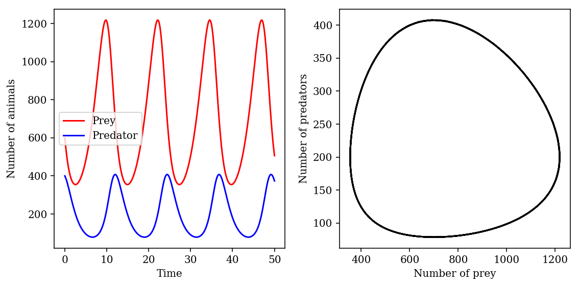
Lotka-Volterra equations for predator/pray populations
$$ x'(t) = a x - b x y $$
$$ y'(t) = c x y - d y $$
a, b, c, d = 0.4, 0.002, 0.001, 0.7
def f(xy, t):
    x, y = xy
    return [a * x - b * x * y,
            c * x * y - d * y]
xy0 = [600, 400]
t = np.linspace(0, 50, 250)
xy_t = integrate.odeint(f, xy0, t)
xy_t.shape
$\displaystyle \left( 250, \ 2\right)$
fig, axes = plt.subplots(1, 2, figsize=(8, 4))

axes[0].plot(t, xy_t[:,0], 'r', label="Prey")
axes[0].plot(t, xy_t[:,1], 'b', label="Predator")
axes[0].set_xlabel("Time")
axes[0].set_ylabel("Number of animals")
axes[0].legend()

axes[1].plot(xy_t[:,0], xy_t[:,1], 'k')
axes[1].set_xlabel("Number of prey")
axes[1].set_ylabel("Number of predators")
fig.tight_layout()
fig.savefig('ch9-lokta-volterra.pdf')
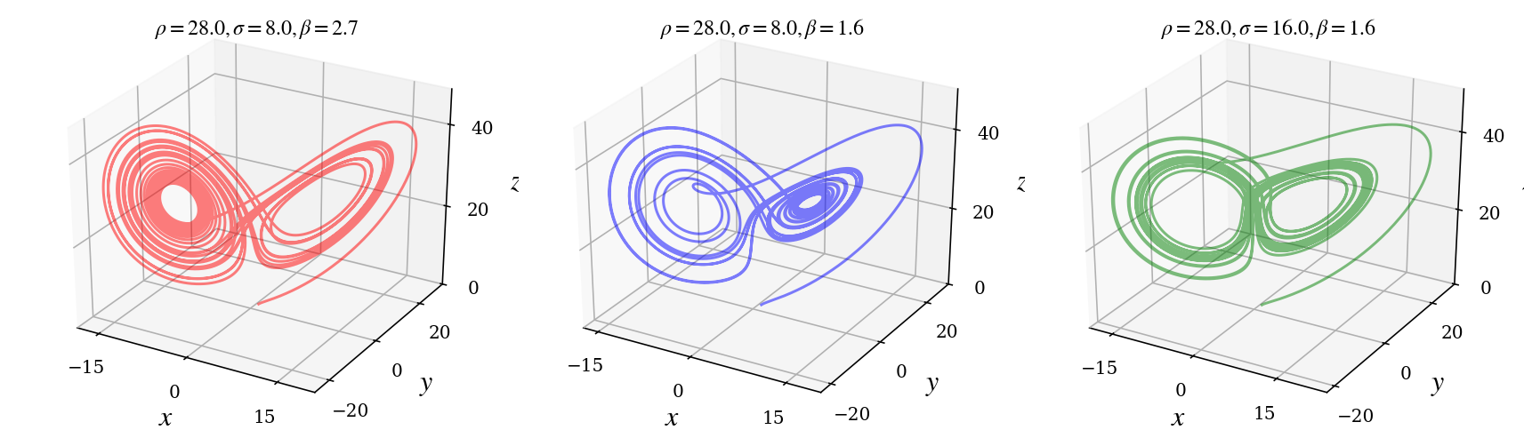
Lorenz equations
$$ x'(t) = \sigma(y - x) $$ $$ y'(t) = x(\rho - z) - y $$ $$ z'(t) = x y - \beta z $$
def f(xyz, t, rho, sigma, beta):
    x, y, z = xyz
    return [sigma * (y - x),
            x * (rho - z) - y,
            x * y - beta * z]
rho = 28
sigma = 8
beta = 8/3.0
t = np.linspace(0, 25, 10000)
xyz0 = [1.0, 1.0, 1.0]
xyz1 = integrate.odeint(f, xyz0, t, args=(rho, sigma, beta))
xyz2 = integrate.odeint(f, xyz0, t, args=(rho, sigma, 0.6*beta))
xyz3 = integrate.odeint(f, xyz0, t, args=(rho, 2*sigma, 0.6*beta))
xyz3.shape
$\displaystyle \left( 10000, \ 3\right)$
from mpl_toolkits.mplot3d.axes3d import Axes3D
fig, (ax1, ax2, ax3) = plt.subplots(1, 3, figsize=(12, 3.5), subplot_kw={'projection': '3d'})

for ax, xyz, c, p in [(ax1, xyz1, 'r', (rho, sigma, beta)),
                      (ax2, xyz2, 'b', (rho, sigma, 0.6*beta)),
                      (ax3, xyz3, 'g', (rho, 2*sigma, 0.6*beta))]:
    ax.plot(xyz[:,0], xyz[:,1], xyz[:,2], c, alpha=0.5)
    ax.set_xlabel('$x$', fontsize=16)
    ax.set_ylabel('$y$', fontsize=16)
    ax.set_zlabel('$z$', fontsize=16)
    ax.set_xticks([-15, 0, 15])
    ax.set_yticks([-20, 0, 20])
    ax.set_zticks([0, 20, 40])
    ax.set_title(r"$\rho=%.1f, \sigma=%.1f, \beta=%.1f$" % (p[0], p[1], p[2]))

fig.tight_layout()
fig.savefig('ch9-lorenz-equations.pdf')
Coupled damped springs
As second-order equations:
\begin{eqnarray}
m_1 x_1''(t) + \gamma_1 x_1'(t) + k_1 (x_1(t) - l_1) - k_2 (x_2(t) - x_1(t) - l_2) &=& 0\
m_2 x_2''(t) + \gamma_2 x_2' + k_2 (x_2 - x_1 - l_2) &=& 0
\end{eqnarray}
On standard form:
\begin{align}
y_1'(t) &= y_2(t) \
y_2'(t) &= -\gamma_1/m_1 y_2(t) - k_1/m_1 (y_1(t) - l_1) + k_2 (y_3(t) - y_1(t) - l_2)/m_1 \
y_3'(t) &= y_4(t) \
y_4'(t) &= - \gamma_2 y_4(t)/m_2 - k_2 (y_3(t) - y_1(t) - l_2)/m_2 \
\end{align}
def f(t, y, args):
    m1, k1, g1, m2, k2, g2 = args

    return [y[1],
            - k1/m1 * y[0] + k2/m1 * (y[2] - y[0]) - g1/m1 * y[1],
            y[3],
            - k2/m2 * (y[2] - y[0]) - g2/m2 * y[3] ]
m1, k1, g1 = 1.0, 10.0, 0.5
m2, k2, g2 = 2.0, 40.0, 0.25
args = (m1, k1, g1, m2, k2, g2)
y0 = [1.0, 0, 0.5, 0]
t = np.linspace(0, 20, 1000)
r = integrate.ode(f)
r.set_integrator('lsoda');
r.set_initial_value(y0, t[0]);
r.set_f_params(args);
dt = t[1] - t[0]
y = np.zeros((len(t), len(y0)))
idx = 0
while r.successful() and r.t < t[-1]:
    y[idx, :] = r.y
    r.integrate(r.t + dt)
    idx += 1
fig = plt.figure(figsize=(10, 4))
ax1 = plt.subplot2grid((2, 5), (0, 0), colspan=3)
ax2 = plt.subplot2grid((2, 5), (1, 0), colspan=3)
ax3 = plt.subplot2grid((2, 5), (0, 3), colspan=2, rowspan=2)

ax1.plot(t, y[:, 0], 'r')
ax1.set_ylabel('$x_1$', fontsize=18)
ax1.set_yticks([-1, -.5, 0, .5, 1])

ax2.plot(t, y[:, 2], 'b')
ax2.set_xlabel('$t$', fontsize=18)
ax2.set_ylabel('$x_2$', fontsize=18)
ax2.set_yticks([-1, -.5, 0, .5, 1])

ax3.plot(y[:, 0], y[:, 2], 'k')
ax3.set_xlabel('$x_1$', fontsize=18)
ax3.set_ylabel('$x_2$', fontsize=18)
ax3.set_xticks([-1, -.5, 0, .5, 1])
ax3.set_yticks([-1, -.5, 0, .5, 1])

fig.tight_layout()
fig.savefig('ch9-coupled-damped-springs.pdf')

Same calculation as above, but with specifying the Jacobian as well:
def jac(t, y, args):
    m1, k1, g1, m2, k2, g2 = args

    return [[0, 1, 0, 0],
            [- k1/m1 - k2/m1, - g1/m1 * y[1], k2/m1, 0],
            [0, 0, 1, 0],
            [k2/m2, 0, - k2/m2, - g2/m2]]
r = integrate.ode(f, jac).set_f_params(args).set_jac_params(args).set_initial_value(y0, t[0])
dt = t[1] - t[0]
y = np.zeros((len(t), len(y0)))
idx = 0
while r.successful() and r.t < t[-1]:
    y[idx, :] = r.y
    r.integrate(r.t + dt)
    idx += 1
fig = plt.figure(figsize=(10, 4))
ax1 = plt.subplot2grid((2, 5), (0, 0), colspan=3)
ax2 = plt.subplot2grid((2, 5), (1, 0), colspan=3)
ax3 = plt.subplot2grid((2, 5), (0, 3), colspan=2, rowspan=2)

ax1.plot(t, y[:, 0], 'r')
ax1.set_ylabel('$x_1$', fontsize=18)
ax1.set_yticks([-1, -.5, 0, .5, 1])

ax2.plot(t, y[:, 2], 'b')
ax2.set_xlabel('$t$', fontsize=18)
ax2.set_ylabel('$x_2$', fontsize=18)
ax2.set_yticks([-1, -.5, 0, .5, 1])

ax3.plot(y[:, 0], y[:, 2], 'k')
ax3.set_xlabel('$x_1$', fontsize=18)
ax3.set_ylabel('$x_2$', fontsize=18)
ax3.set_xticks([-1, -.5, 0, .5, 1])
ax3.set_yticks([-1, -.5, 0, .5, 1])

fig.tight_layout()
Same calculation, but using SymPy to setup the problem for SciPy
L1 = L2 = 0
t = sympy.symbols("t")
m1, k1, b1 = sympy.symbols("m_1, k_1, b_1")
m2, k2, b2 = sympy.symbols("m_2, k_2, b_2")
x1 = sympy.Function("x_1")
x2 = sympy.Function("x_2")
ode1 = sympy.Eq(m1 * x1(t).diff(t,t,) + b1 * x1(t).diff(t) + k1*(x1(t)-L1) - k2*(x2(t)-x1(t) - L2))
ode2 = sympy.Eq(m2 * x2(t).diff(t,t,) + b2 * x2(t).diff(t) + k2*(x2(t)-x1(t)-L2))
params = {m1: 1.0, k1: 10.0, b1: 0.5,
          m2: 2.0, k2: 40.0, b2: 0.25}
args
$\displaystyle \left( 1.0, \ 10.0, \ 0.5, \ 2.0, \ 40.0, \ 0.25\right)$
y1 = sympy.Function("y_1")
y2 = sympy.Function("y_2")
y3 = sympy.Function("y_3")
y4 = sympy.Function("y_4")
varchange = {x1(t).diff(t, t): y2(t).diff(t),
             x1(t): y1(t),
             x2(t).diff(t, t): y4(t).diff(t),
             x2(t): y3(t)}
(ode1.subs(varchange).lhs, ode2.subs(varchange).lhs)
$\displaystyle \left( b_{1} \frac{d}{d t} \operatorname{y_{1}}{\left(t \right)} + k_{1} \operatorname{y_{1}}{\left(t \right)} - k_{2} \left(- \operatorname{y_{1}}{\left(t \right)} + \operatorname{y_{3}}{\left(t \right)}\right) + m_{1} \frac{d}{d t} \operatorname{y_{2}}{\left(t \right)}, \ b_{2} \frac{d}{d t} \operatorname{y_{3}}{\left(t \right)} + k_{2} \left(- \operatorname{y_{1}}{\left(t \right)} + \operatorname{y_{3}}{\left(t \right)}\right) + m_{2} \frac{d}{d t} \operatorname{y_{4}}{\left(t \right)}\right)$
ode3 = y1(t).diff(t) - y2(t)
ode4 = y3(t).diff(t) - y4(t)
vcsol = sympy.solve((ode1.subs(varchange), ode2.subs(varchange), ode3, ode4),
                    (y1(t).diff(t), y2(t).diff(t), y3(t).diff(t), y4(t).diff(t)))
vcsol
$\displaystyle \left{ \frac{d}{d t} \operatorname{y_{1}}{\left(t \right)} : \operatorname{y_{2}}{\left(t \right)}, \ \frac{d}{d t} \operatorname{y_{2}}{\left(t \right)} : \frac{- b_{1} \operatorname{y_{2}}{\left(t \right)} - k_{1} \operatorname{y_{1}}{\left(t \right)} - k_{2} \operatorname{y_{1}}{\left(t \right)} + k_{2} \operatorname{y_{3}}{\left(t \right)}}{m_{1}}, \ \frac{d}{d t} \operatorname{y_{3}}{\left(t \right)} : \operatorname{y_{4}}{\left(t \right)}, \ \frac{d}{d t} \operatorname{y_{4}}{\left(t \right)} : \frac{- b_{2} \operatorname{y_{4}}{\left(t \right)} + k_{2} \operatorname{y_{1}}{\left(t \right)} - k_{2} \operatorname{y_{3}}{\left(t \right)}}{m_{2}}\right}$
ode_rhs = sympy.Matrix([y1(t).diff(t), y2(t).diff(t), y3(t).diff(t), y4(t).diff(t)]).subs(vcsol)
y = sympy.Matrix([y1(t), y2(t), y3(t), y4(t)])
sympy.Eq(y.diff(t), ode_rhs)
$\displaystyle \left[\begin{matrix}\frac{d}{d t} \operatorname{y_{1}}{\left(t \right)}\\frac{d}{d t} \operatorname{y_{2}}{\left(t \right)}\\frac{d}{d t} \operatorname{y_{3}}{\left(t \right)}\\frac{d}{d t} \operatorname{y_{4}}{\left(t \right)}\end{matrix}\right] = \left[\begin{matrix}\operatorname{y_{2}}{\left(t \right)}\\frac{- b_{1} \operatorname{y_{2}}{\left(t \right)} - k_{1} \operatorname{y_{1}}{\left(t \right)} - k_{2} \operatorname{y_{1}}{\left(t \right)} + k_{2} \operatorname{y_{3}}{\left(t \right)}}{m_{1}}\\operatorname{y_{4}}{\left(t \right)}\\frac{- b_{2} \operatorname{y_{4}}{\left(t \right)} + k_{2} \operatorname{y_{1}}{\left(t \right)} - k_{2} \operatorname{y_{3}}{\left(t \right)}}{m_{2}}\end{matrix}\right]$
ode_rhs.subs(params)
$\displaystyle \left[\begin{matrix}\operatorname{y_{2}}{\left(t \right)}\- 50.0 \operatorname{y_{1}}{\left(t \right)} - 0.5 \operatorname{y_{2}}{\left(t \right)} + 40.0 \operatorname{y_{3}}{\left(t \right)}\\operatorname{y_{4}}{\left(t \right)}\20.0 \operatorname{y_{1}}{\left(t \right)} - 20.0 \operatorname{y_{3}}{\left(t \right)} - 0.125 \operatorname{y_{4}}{\left(t \right)}\end{matrix}\right]$
_f_np = sympy.lambdify((t, y), ode_rhs.subs(params), 'numpy')
f_np = lambda _x, _y, *args: _f_np(_x, _y)
y0 = [1.0, 0, 0.5, 0]
tt = np.linspace(0, 20, 1000)

r = integrate.ode(f_np)
r.set_integrator('lsoda');
r.set_initial_value(y0, tt[0]);

dt = tt[1] - tt[0]
yy = np.zeros((len(tt), len(y0)))
idx = 0
while r.successful() and r.t < tt[-1]:
    yy[idx, :] = r.y
    r.integrate(r.t + dt)
    idx += 1
fig = plt.figure(figsize=(10, 4))
ax1 = plt.subplot2grid((2, 5), (0, 0), colspan=3)
ax2 = plt.subplot2grid((2, 5), (1, 0), colspan=3)
ax3 = plt.subplot2grid((2, 5), (0, 3), colspan=2, rowspan=2)

ax1.plot(tt, yy[:, 0], 'r')
ax1.set_ylabel('$x_1$', fontsize=18)
ax1.set_yticks([-1, -.5, 0, .5, 1])

ax2.plot(tt, yy[:, 2], 'b')
ax2.set_xlabel('$t$', fontsize=18)
ax2.set_ylabel('$x_2$', fontsize=18)
ax2.set_yticks([-1, -.5, 0, .5, 1])

ax3.plot(yy[:, 0], yy[:, 2], 'k')
ax3.set_xlabel('$x_1$', fontsize=18)
ax3.set_ylabel('$x_2$', fontsize=18)
ax3.set_xticks([-1, -.5, 0, .5, 1])
ax3.set_yticks([-1, -.5, 0, .5, 1])

fig.tight_layout()

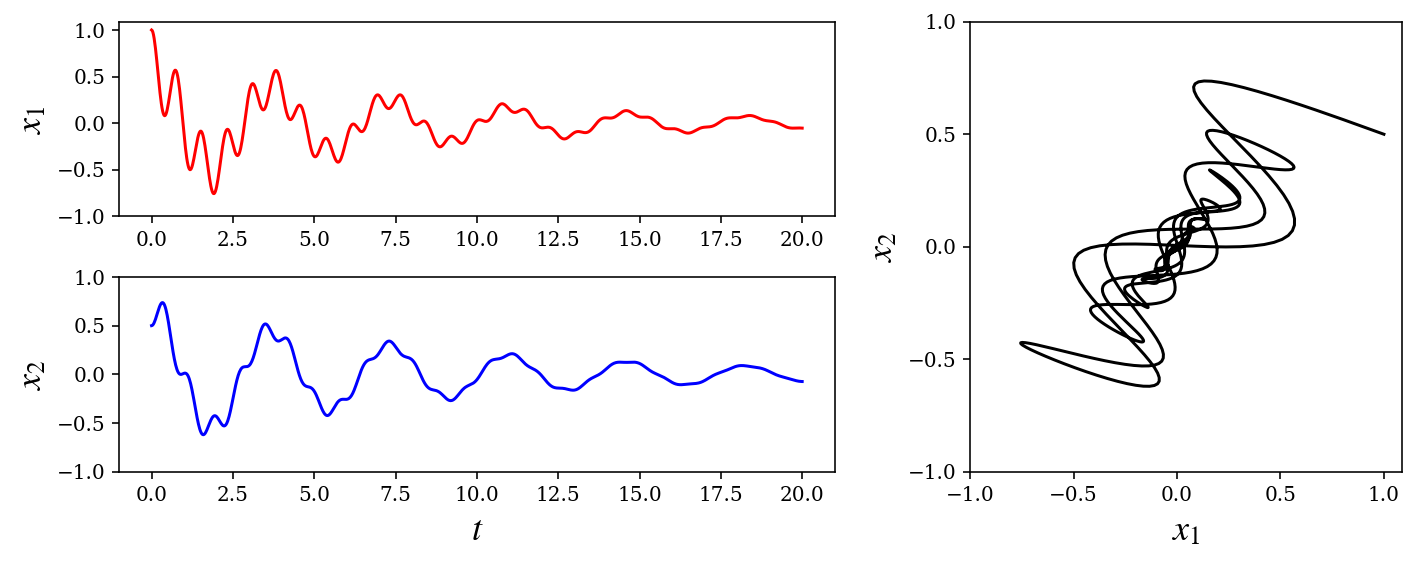
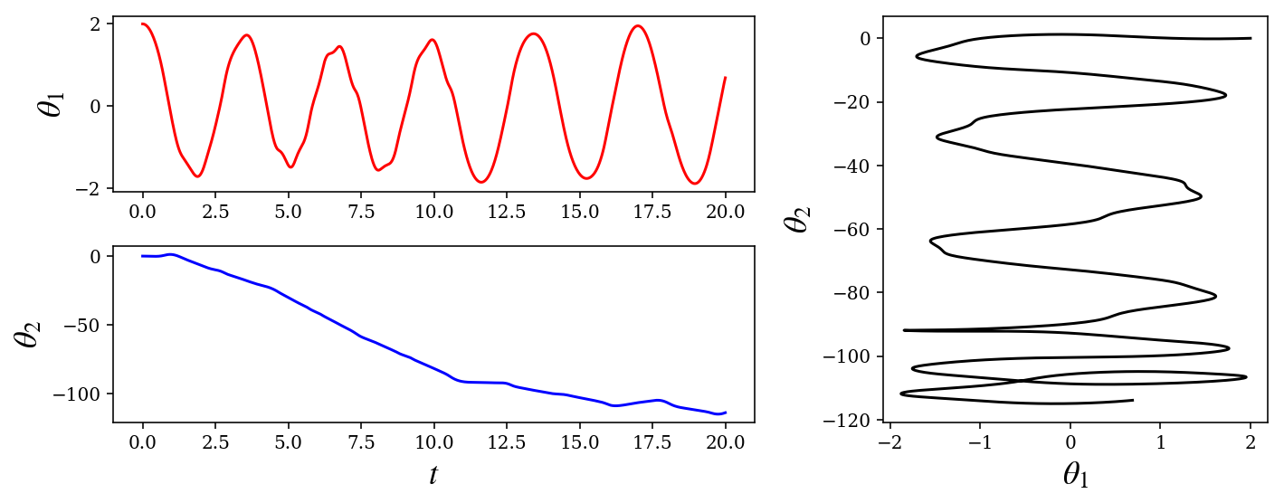
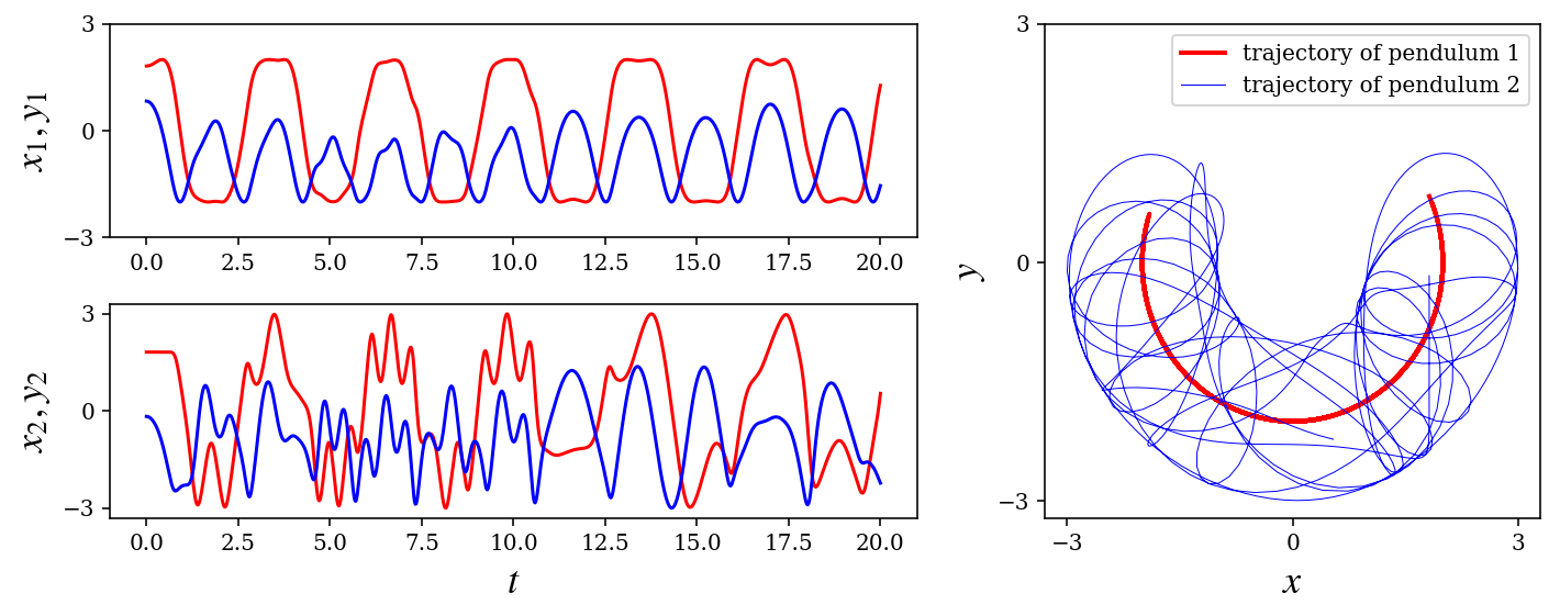
Doube pendulum
http://scienceworld.wolfram.com/physics/DoublePendulum.html
$$ (m_1+m_2) l_1\theta_1'' + m_2l_2\theta_2''\cos(\theta_1-\theta_2)
- m_2l_2(\theta_2')^2\sin(\theta_1-\theta_2)+g(m_1+m_2)\sin(\theta_1) = 0 $$
$$ m_2l_2\theta_2'' + m_2l_1\theta_1''\cos(\theta_1-\theta_2) - m_2l_1 (\theta_1')^2 \sin(\theta_1-\theta_2) +m_2g\sin(\theta_2) = 0 $$
t, g, m1, l1, m2, l2 = sympy.symbols("t, g, m_1, l_1, m_2, l_2")
theta1, theta2 = sympy.symbols("theta_1, theta_2", cls=sympy.Function)
ode1 = sympy.Eq((m1+m2)*l1 * theta1(t).diff(t,t) +
                m2*l2 * theta2(t).diff(t,t) * sympy.cos(theta1(t)-theta2(t))  +
                m2*l2 * theta2(t).diff(t)**2 * sympy.sin(theta1(t)-theta2(t)) +
                g*(m1+m2) * sympy.sin(theta1(t)))
ode1
$\displaystyle g \left(m_{1} + m_{2}\right) \sin{\left(\theta_{1}{\left(t \right)} \right)} + l_{1} \left(m_{1} + m_{2}\right) \frac{d^{2}}{d t^{2}} \theta_{1}{\left(t \right)} + l_{2} m_{2} \sin{\left(\theta_{1}{\left(t \right)} - \theta_{2}{\left(t \right)} \right)} \left(\frac{d}{d t} \theta_{2}{\left(t \right)}\right)^{2} + l_{2} m_{2} \cos{\left(\theta_{1}{\left(t \right)} - \theta_{2}{\left(t \right)} \right)} \frac{d^{2}}{d t^{2}} \theta_{2}{\left(t \right)} = 0$
ode2 = sympy.Eq(m2*l2 * theta2(t).diff(t,t) +
                m2*l1 * theta1(t).diff(t,t) * sympy.cos(theta1(t)-theta2(t)) -
                m2*l1 * theta1(t).diff(t)**2 * sympy.sin(theta1(t) - theta2(t)) +
                m2*g * sympy.sin(theta2(t)))
ode2
$\displaystyle g m_{2} \sin{\left(\theta_{2}{\left(t \right)} \right)} - l_{1} m_{2} \sin{\left(\theta_{1}{\left(t \right)} - \theta_{2}{\left(t \right)} \right)} \left(\frac{d}{d t} \theta_{1}{\left(t \right)}\right)^{2} + l_{1} m_{2} \cos{\left(\theta_{1}{\left(t \right)} - \theta_{2}{\left(t \right)} \right)} \frac{d^{2}}{d t^{2}} \theta_{1}{\left(t \right)} + l_{2} m_{2} \frac{d^{2}}{d t^{2}} \theta_{2}{\left(t \right)} = 0$
# this is fruitless, sympy cannot solve these ODEs
try:
    sympy.dsolve(ode1, ode2)
except Exception as e:
    print(e)
cannot determine truth value of Relational
y1, y2, y3, y4 = sympy.symbols("y_1, y_2, y_3, y_4", cls=sympy.Function)
varchange = {theta1(t).diff(t, t): y2(t).diff(t),
             theta1(t): y1(t),
             theta2(t).diff(t, t): y4(t).diff(t),
             theta2(t): y3(t)}
ode1_vc = ode1.subs(varchange)
ode2_vc = ode2.subs(varchange)
ode3 = y1(t).diff(t) - y2(t)
ode4 = y3(t).diff(t) - y4(t)
y = sympy.Matrix([y1(t), y2(t), y3(t), y4(t)])
vcsol = sympy.solve((ode1_vc, ode2_vc, ode3, ode4), y.diff(t), dict=True)
f = y.diff(t).subs(vcsol[0])
sympy.Eq(y.diff(t), f)
$\displaystyle \left[\begin{matrix}\frac{d}{d t} \operatorname{y_{1}}{\left(t \right)}\\frac{d}{d t} \operatorname{y_{2}}{\left(t \right)}\\frac{d}{d t} \operatorname{y_{3}}{\left(t \right)}\\frac{d}{d t} \operatorname{y_{4}}{\left(t \right)}\end{matrix}\right] = \left[\begin{matrix}\operatorname{y_{2}}{\left(t \right)}\\frac{g m_{1} \sin{\left(\operatorname{y_{1}}{\left(t \right)} \right)} + \frac{g m_{2} \sin{\left(\operatorname{y_{1}}{\left(t \right)} - 2 \operatorname{y_{3}}{\left(t \right)} \right)}}{2} + \frac{g m_{2} \sin{\left(\operatorname{y_{1}}{\left(t \right)} \right)}}{2} + \frac{l_{1} m_{2} \operatorname{y_{2}}^{2}{\left(t \right)} \sin{\left(2 \operatorname{y_{1}}{\left(t \right)} - 2 \operatorname{y_{3}}{\left(t \right)} \right)}}{2} + l_{2} m_{2} \operatorname{y_{4}}^{2}{\left(t \right)} \sin{\left(\operatorname{y_{1}}{\left(t \right)} - \operatorname{y_{3}}{\left(t \right)} \right)}}{l_{1} \left(- m_{1} + m_{2} \cos^{2}{\left(\operatorname{y_{1}}{\left(t \right)} - \operatorname{y_{3}}{\left(t \right)} \right)} - m_{2}\right)}\\operatorname{y_{4}}{\left(t \right)}\\frac{g m_{1} \sin{\left(2 \operatorname{y_{1}}{\left(t \right)} - \operatorname{y_{3}}{\left(t \right)} \right)} - g m_{1} \sin{\left(\operatorname{y_{3}}{\left(t \right)} \right)} + g m_{2} \sin{\left(2 \operatorname{y_{1}}{\left(t \right)} - \operatorname{y_{3}}{\left(t \right)} \right)} - g m_{2} \sin{\left(\operatorname{y_{3}}{\left(t \right)} \right)} + 2 l_{1} m_{1} \operatorname{y_{2}}^{2}{\left(t \right)} \sin{\left(\operatorname{y_{1}}{\left(t \right)} - \operatorname{y_{3}}{\left(t \right)} \right)} + 2 l_{1} m_{2} \operatorname{y_{2}}^{2}{\left(t \right)} \sin{\left(\operatorname{y_{1}}{\left(t \right)} - \operatorname{y_{3}}{\left(t \right)} \right)} + l_{2} m_{2} \operatorname{y_{4}}^{2}{\left(t \right)} \sin{\left(2 \operatorname{y_{1}}{\left(t \right)} - 2 \operatorname{y_{3}}{\left(t \right)} \right)}}{2 l_{2} \left(m_{1} - m_{2} \cos^{2}{\left(\operatorname{y_{1}}{\left(t \right)} - \operatorname{y_{3}}{\left(t \right)} \right)} + m_{2}\right)}\end{matrix}\right]$
params = {m1: 5.0, l1: 2.0,
          m2: 1.0, l2: 1.0, g: 10.0}
_f_np = sympy.lambdify((t, y), f.subs(params), 'numpy')
f_np = lambda _t, _y, *args: _f_np(_t, _y)
jac = sympy.Matrix([[fj.diff(yi) for yi in y] for fj in f])
_jac_np = sympy.lambdify((t, y), jac.subs(params), 'numpy')
jac_np = lambda _t, _y, *args: _jac_np(_t, _y)
y0 = [2.0, 0, 0.0, 0]
tt = np.linspace(0, 20, 1000)
%%time

r = integrate.ode(f_np, jac_np).set_initial_value(y0, tt[0]);

dt = tt[1] - tt[0]
yy = np.zeros((len(tt), len(y0)))
idx = 0
while r.successful() and r.t < tt[-1]:
    yy[idx, :] = r.y
    r.integrate(r.t + dt)
    idx += 1
CPU times: user 124 ms, sys: 14.1 ms, total: 138 ms
Wall time: 127 ms
fig = plt.figure(figsize=(10, 4))
ax1 = plt.subplot2grid((2, 5), (0, 0), colspan=3)
ax2 = plt.subplot2grid((2, 5), (1, 0), colspan=3)
ax3 = plt.subplot2grid((2, 5), (0, 3), colspan=2, rowspan=2)

ax1.plot(tt, yy[:, 0], 'r')
ax1.set_ylabel(r'$\theta_1$', fontsize=18)

ax2.plot(tt, yy[:, 2], 'b')
ax2.set_xlabel('$t$', fontsize=18)
ax2.set_ylabel(r'$\theta_2$', fontsize=18)

ax3.plot(yy[:, 0], yy[:, 2], 'k')
ax3.set_xlabel(r'$\theta_1$', fontsize=18)
ax3.set_ylabel(r'$\theta_2$', fontsize=18)

fig.tight_layout()
theta1_np, theta2_np = yy[:, 0], yy[:, 2]
x1 = params[l1] * np.sin(theta1_np)
y1 = -params[l1] * np.cos(theta1_np)
x2 = x1 + params[l2] * np.sin(theta2_np)
y2 = y1 - params[l2] * np.cos(theta2_np)
fig = plt.figure(figsize=(10, 4))
ax1 = plt.subplot2grid((2, 5), (0, 0), colspan=3)
ax2 = plt.subplot2grid((2, 5), (1, 0), colspan=3)
ax3 = plt.subplot2grid((2, 5), (0, 3), colspan=2, rowspan=2)

ax1.plot(tt, x1, 'r')
ax1.plot(tt, y1, 'b')
ax1.set_ylabel('$x_1, y_1$', fontsize=18)
ax1.set_yticks([-3, 0, 3])

ax2.plot(tt, x2, 'r')
ax2.plot(tt, y2, 'b')
ax2.set_xlabel('$t$', fontsize=18)
ax2.set_ylabel('$x_2, y_2$', fontsize=18)
ax2.set_yticks([-3, 0, 3])

ax3.plot(x1, y1, 'r', lw=2.0, label="trajectory of pendulum 1")
ax3.plot(x2, y2, 'b', lw=0.5, label="trajectory of pendulum 2")
ax3.set_xlabel('$x$', fontsize=18)
ax3.set_ylabel('$y$', fontsize=18)
ax3.set_xticks([-3, 0, 3])
ax3.set_yticks([-3, 0, 3])
ax3.legend()

fig.tight_layout()
fig.savefig('ch9-double-pendulum.pdf')
Versions
%reload_ext version_information
%version_information numpy, scipy, sympy, matplotlib