Jupyter Snippet NP ch07-code-listing
Jupyter Snippet NP ch07-code-listing
Chapter 7: Interpolation
Robert Johansson
Source code listings for Numerical Python - Scientific Computing and Data Science Applications with Numpy, SciPy and Matplotlib (ISBN 978-1-484242-45-2).
%matplotlib inline

import matplotlib as mpl
mpl.rcParams["font.family"] = "serif"
mpl.rcParams["font.size"] = "12"

mpl.rcParams['mathtext.fontset'] = 'stix'
mpl.rcParams['font.family'] = 'serif'
mpl.rcParams['font.sans-serif'] = 'stix'
import numpy as np
from numpy import polynomial as P
from scipy import interpolate
import matplotlib.pyplot as plt
from scipy import linalg
Polynomials
p1 = P.Polynomial([1,2,3])
p1
$x \mapsto \text{1.0} + \text{2.0},x + \text{3.0},x^{2}$
p2 = P.Polynomial.fromroots([-1, 1])
p2
$x \mapsto \text{-1.0}\color{LightGray}{ + \text{0.0},x} + \text{1.0},x^{2}$
p1.roots()
array([-0.33333333-0.47140452j, -0.33333333+0.47140452j])
p2.roots()
array([-1., 1.])
p1.coef
array([1., 2., 3.])
p1.domain
array([-1, 1])
p1.window
array([-1, 1])
p1(np.array([1.5, 2.5, 3.5]))
array([10.75, 24.75, 44.75])
# p1([1.5, 2.5, 3.5])
p1+p2
$x \mapsto \color{LightGray}{\text{0.0}} + \text{2.0},x + \text{4.0},x^{2}$
p2 / 5
$x \mapsto \text{-0.2}\color{LightGray}{ + \text{0.0},x} + \text{0.2},x^{2}$
p1 = P.Polynomial.fromroots([1, 2, 3])
p1
$x \mapsto \text{-6.0} + \text{11.0},x - \text{6.0},x^{2} + \text{1.0},x^{3}$
p2 = P.Polynomial.fromroots([2])
p2
$x \mapsto \text{-2.0} + \text{1.0},x$
p3 = p1 // p2
p3
$x \mapsto \text{3.0} - \text{4.0},x + \text{1.0},x^{2}$
p3.roots()
array([1., 3.])
p2
$x \mapsto \text{-2.0} + \text{1.0},x$
c1 = P.Chebyshev([1, 2, 3])
c1
$x \mapsto \text{1.0},{T}{0}(x) + \text{2.0},{T}{1}(x) + \text{3.0},{T}_{2}(x)$
c1.roots()
array([-0.76759188, 0.43425855])
c = P.Chebyshev.fromroots([-1, 1])
c
$x \mapsto \text{-0.5},{T}{0}(x)\color{LightGray}{ + \text{0.0},{T}{1}(x)} + \text{0.5},{T}_{2}(x)$
l = P.Legendre.fromroots([-1, 1])
l
$x \mapsto \text{-0.6666666666666667},{P}{0}(x)\color{LightGray}{ + \text{0.0},{P}{1}(x)} + \text{0.6666666666666666},{P}_{2}(x)$
c(np.array([0.5, 1.5, 2.5]))
array([-0.75, 1.25, 5.25])
l(np.array([0.5, 1.5, 2.5]))
array([-0.75, 1.25, 5.25])
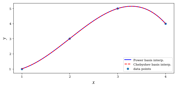
Polynomial interpolation
x = np.array([1, 2, 3, 4])
y = np.array([1, 3, 5, 4])
deg = len(x) - 1
A = P.polynomial.polyvander(x, deg)
c = linalg.solve(A, y)
c
array([ 2. , -3.5, 3. , -0.5])
f1 = P.Polynomial(c)
f1(2.5)
4.1875
A = P.chebyshev.chebvander(x, deg)
c = linalg.solve(A, y)
c
array([ 3.5 , -3.875, 1.5 , -0.125])
f2 = P.Chebyshev(c)
f2(2.5)
4.1875
xx = np.linspace(x.min(), x.max(), 100)

fig, ax = plt.subplots(1, 1, figsize=(8, 4))

ax.plot(xx, f1(xx), 'b', lw=2, label='Power basis interp.')
ax.plot(xx, f2(xx), 'r--', lw=2, label='Chebyshev basis interp.')
ax.scatter(x, y, label='data points')

ax.legend(loc=4)
ax.set_xticks(x)
ax.set_ylabel(r"$y$", fontsize=18)
ax.set_xlabel(r"$x$", fontsize=18)

fig.tight_layout()
fig.savefig('ch7-polynomial-interpolation.pdf');
f1b = P.Polynomial.fit(x, y, deg)
f1b
$x \mapsto \text{4.187500000000003} + \text{3.187499999999996},\left(\text{-1.6666666666666667} + \text{0.6666666666666666}x\right) - \text{1.687500000000004},\left(\text{-1.6666666666666667} + \text{0.6666666666666666}x\right)^{2} - \text{1.6874999999999973},\left(\text{-1.6666666666666667} + \text{0.6666666666666666}x\right)^{3}$
f2b = P.Chebyshev.fit(x, y, deg)
f2b
$x \mapsto \text{3.3437500000000004},{T}{0}(\text{-1.6666666666666667} + \text{0.6666666666666666}x) + \text{1.9218749999999991},{T}{1}(\text{-1.6666666666666667} + \text{0.6666666666666666}x) - \text{0.8437500000000021},{T}{2}(\text{-1.6666666666666667} + \text{0.6666666666666666}x) - \text{0.42187499999999944},{T}{3}(\text{-1.6666666666666667} + \text{0.6666666666666666}x)$
np.linalg.cond(P.chebyshev.chebvander(x, deg))
4659.738424139959
np.linalg.cond(P.chebyshev.chebvander((2*x-5)/3.0, deg))
1.8542033440472896
(2 * x - 5)/3.0
array([-1. , -0.33333333, 0.33333333, 1. ])
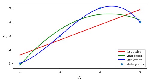
f1 = P.Polynomial.fit(x, y, 1)
f2 = P.Polynomial.fit(x, y, 2)
f3 = P.Polynomial.fit(x, y, 3)
xx = np.linspace(x.min(), x.max(), 100)

fig, ax = plt.subplots(1, 1, figsize=(8, 4))

ax.plot(xx, f1(xx), 'r', lw=2, label='1st order')
ax.plot(xx, f2(xx), 'g', lw=2, label='2nd order')
ax.plot(xx, f3(xx), 'b', lw=2, label='3rd order')
ax.scatter(x, y, label='data points')

ax.legend(loc=4)
ax.set_xticks(x)
ax.set_ylabel(r"$y$", fontsize=18)
ax.set_xlabel(r"$x$", fontsize=18);
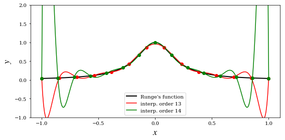
Runge problem
def runge(x):
    return 1/(1 + 25 * x**2)
def runge_interpolate(n):
    x = np.linspace(-1, 1, n + 1)
    p = P.Polynomial.fit(x, runge(x), deg=n)
    return x, p
xx = np.linspace(-1, 1, 250)
fig, ax = plt.subplots(1, 1, figsize=(8, 4))

ax.plot(xx, runge(xx), 'k', lw=2, label="Runge's function")

n = 13
x, p = runge_interpolate(n)
ax.plot(x, runge(x), 'ro')
ax.plot(xx, p(xx), 'r', label='interp. order %d' % n)

n = 14
x, p = runge_interpolate(n)
ax.plot(x, runge(x), 'go')
ax.plot(xx, p(xx), 'g', label='interp. order %d' % n)

ax.legend(loc=8)
ax.set_xlim(-1.1, 1.1)
ax.set_ylim(-1, 2)
ax.set_xticks([-1, -0.5, 0, 0.5, 1])
ax.set_ylabel(r"$y$", fontsize=18)
ax.set_xlabel(r"$x$", fontsize=18)

fig.tight_layout()
fig.savefig('ch7-polynomial-interpolation-runge.pdf');
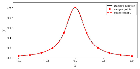
Spline interpolation
x = np.linspace(-1, 1, 11)
y = runge(x)
f = interpolate.interp1d(x, y, kind=3)
xx = np.linspace(-1, 1, 100)
fig, ax = plt.subplots(figsize=(8, 4))

ax.plot(xx, runge(xx), 'k', lw=1, label="Runge's function")
ax.plot(x, y, 'ro', label='sample points')
ax.plot(xx, f(xx), 'r--', lw=2, label='spline order 3')

ax.legend()
ax.set_ylim(0, 1.1)
ax.set_xticks([-1, -0.5, 0, 0.5, 1])
ax.set_ylabel(r"$y$", fontsize=18)
ax.set_xlabel(r"$x$", fontsize=18)

fig.tight_layout()
fig.savefig('ch7-spline-interpolation-runge.pdf');
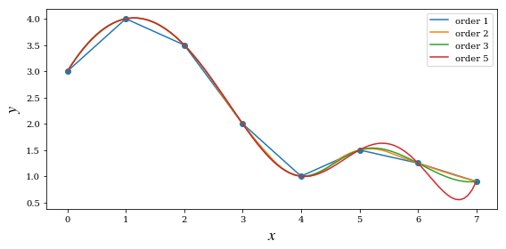
x = np.array([0, 1, 2, 3, 4, 5, 6, 7])
y = np.array([3, 4, 3.5, 2, 1, 1.5, 1.25, 0.9])
xx = np.linspace(x.min(), x.max(), 100)
fig, ax = plt.subplots(figsize=(8, 4))

ax.scatter(x, y)

for n in [1, 2, 3, 5]:
    f = interpolate.interp1d(x, y, kind=n)
    ax.plot(xx, f(xx), label='order %d' % n)

ax.legend()
ax.set_ylabel(r"$y$", fontsize=18)
ax.set_xlabel(r"$x$", fontsize=18)

fig.tight_layout()
fig.savefig('ch7-spline-interpolation-orders.pdf');
Multivariate interpolation
Regular grid
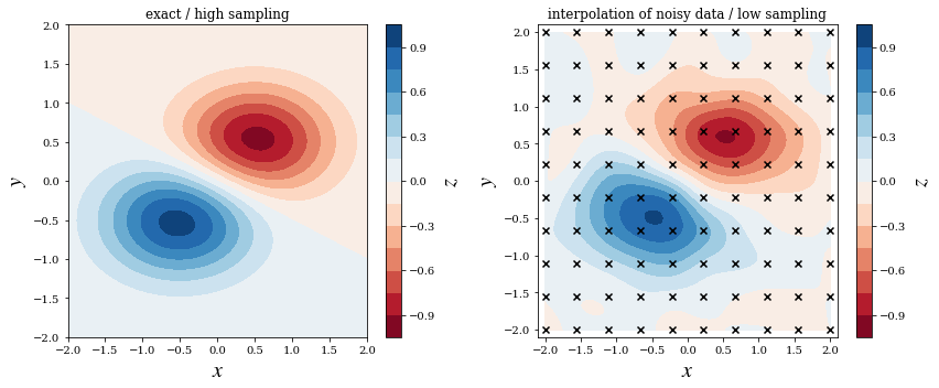
x = y = np.linspace(-2, 2, 10)
def f(x, y):
    return np.exp(-(x + .5)**2 - 2*(y + .5)**2) - np.exp(-(x - .5)**2 - 2*(y - .5)**2)
X, Y = np.meshgrid(x, y)
# simulate noisy data at fixed grid points X, Y
Z = f(X, Y) + 0.05 * np.random.randn(*X.shape)
f_interp = interpolate.interp2d(x, y, Z, kind='cubic')
xx = yy = np.linspace(x.min(), x.max(), 100)
ZZi = f_interp(xx, yy)
XX, YY = np.meshgrid(xx, yy)
fig, axes = plt.subplots(1, 2, figsize=(12, 5))

c = axes[0].contourf(XX, YY, f(XX, YY), 15, cmap=plt.cm.RdBu)
axes[0].set_xlabel(r"$x$", fontsize=20)
axes[0].set_ylabel(r"$y$", fontsize=20)
axes[0].set_title("exact / high sampling")
cb = fig.colorbar(c, ax=axes[0])
cb.set_label(r"$z$", fontsize=20)

c = axes[1].contourf(XX, YY, ZZi, 15, cmap=plt.cm.RdBu)
axes[1].set_ylim(-2.1, 2.1)
axes[1].set_xlim(-2.1, 2.1)
axes[1].set_xlabel(r"$x$", fontsize=20)
axes[1].set_ylabel(r"$y$", fontsize=20)
axes[1].scatter(X, Y, marker='x', color='k')
axes[1].set_title("interpolation of noisy data / low sampling")
cb = fig.colorbar(c, ax=axes[1])
cb.set_label(r"$z$", fontsize=20)

fig.tight_layout()
fig.savefig('ch7-multivariate-interpolation-regular-grid.pdf')
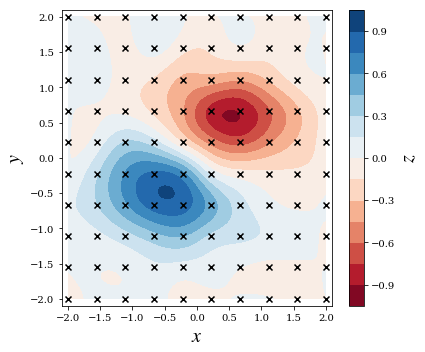
fig, ax = plt.subplots(1, 1, figsize=(6, 5))

c = ax.contourf(XX, YY, ZZi, 15, cmap=plt.cm.RdBu)
ax.set_ylim(-2.1, 2.1)
ax.set_xlim(-2.1, 2.1)
ax.set_xlabel(r"$x$", fontsize=20)
ax.set_ylabel(r"$y$", fontsize=20)
ax.scatter(X, Y, marker='x', color='k')
cb = fig.colorbar(c, ax=ax)
cb.set_label(r"$z$", fontsize=20)

fig.tight_layout()
#fig.savefig('ch7-multivariate-interpolation-regular-grid.pdf')
Irregular grid
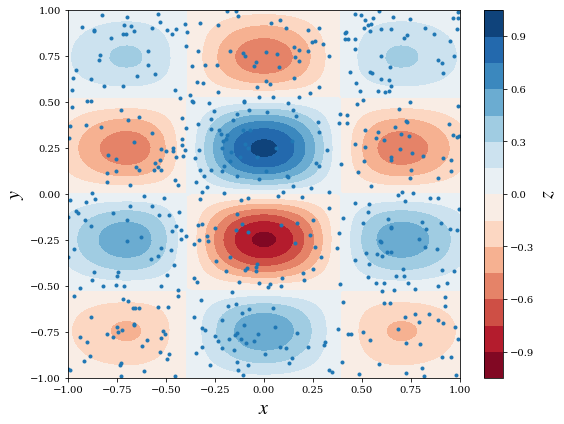
np.random.seed(115925231)
x = y = np.linspace(-1, 1, 100)
X, Y = np.meshgrid(x, y)
def f(x, y):
    return np.exp(-x**2 - y**2) * np.cos(4*x) * np.sin(6*y)
Z = f(X, Y)
N = 500
xdata = np.random.uniform(-1, 1, N)
ydata = np.random.uniform(-1, 1, N)
zdata = f(xdata, ydata)
fig, ax = plt.subplots(figsize=(8, 6))
c = ax.contourf(X, Y, Z, 15, cmap=plt.cm.RdBu);
ax.scatter(xdata, ydata, marker='.')
ax.set_ylim(-1,1)
ax.set_xlim(-1,1)
ax.set_xlabel(r"$x$", fontsize=20)
ax.set_ylabel(r"$y$", fontsize=20)

cb = fig.colorbar(c, ax=ax)
cb.set_label(r"$z$", fontsize=20)

fig.tight_layout()
fig.savefig('ch7-multivariate-interpolation-exact.pdf');
def z_interpolate(xdata, ydata, zdata):
    Zi_0 = interpolate.griddata((xdata, ydata), zdata, (X, Y), method='nearest')
    Zi_1 = interpolate.griddata((xdata, ydata), zdata, (X, Y), method='linear')
    Zi_3 = interpolate.griddata((xdata, ydata), zdata, (X, Y), method='cubic')
    return Zi_0, Zi_1, Zi_3
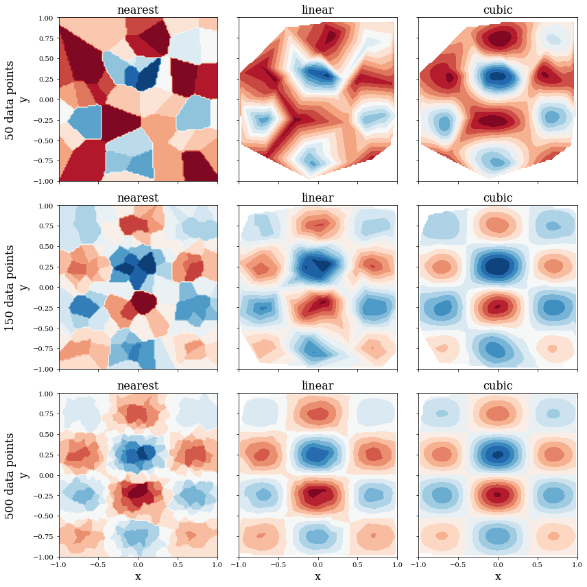
fig, axes = plt.subplots(3, 3, figsize=(12, 12), sharex=True, sharey=True)

n_vec = [50, 150, 500]

for idx, n in enumerate(n_vec):
    Zi_0, Zi_1, Zi_3 = z_interpolate(xdata[:n], ydata[:n], zdata[:n])
    axes[idx, 0].contourf(X, Y, Zi_0, 15, cmap=plt.cm.RdBu)
    axes[idx, 0].set_ylabel("%d data points\ny" % n, fontsize=16)
    axes[idx, 0].set_title("nearest", fontsize=16)
    axes[idx, 1].contourf(X, Y, Zi_1, 15, cmap=plt.cm.RdBu)
    axes[idx, 1].set_title("linear", fontsize=16)
    axes[idx, 2].contourf(X, Y, Zi_3, 15, cmap=plt.cm.RdBu)
    axes[idx, 2].set_title("cubic", fontsize=16)

for m in range(len(n_vec)):
    axes[idx, m].set_xlabel("x", fontsize=16)

fig.tight_layout()
fig.savefig('ch7-multivariate-interpolation-interp.pdf');
Versions
%reload_ext version_information
%version_information scipy, numpy, matplotlib