Jupyter Snippet NP ch05-code-listing
Jupyter Snippet NP ch05-code-listing
Chapter 5: Equation solving
Robert Johansson
Source code listings for Numerical Python - Scientific Computing and Data Science Applications with Numpy, SciPy and Matplotlib (ISBN 978-1-484242-45-2).
%matplotlib inline
import matplotlib.pyplot as plt
import matplotlib
matplotlib.rcParams['mathtext.fontset'] = 'stix'
matplotlib.rcParams['font.family'] = 'serif'
matplotlib.rcParams['font.sans-serif'] = 'stix'
from scipy import linalg as la
from scipy import optimize
import sympy
sympy.init_printing()
import numpy as np
import matplotlib.pyplot as plt
%matplotlib inline

#import matplotlib as mpl
#mpl.rcParams["font.family"] = "serif"
#mpl.rcParams["font.size"] = "12"
from __future__ import division
Linear Algebra - Linear Equation Systems
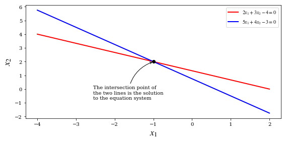
$$ 2 x_1 + 3 x_2 = 4 $$
$$ 5 x_1 + 4 x_2 = 3 $$
fig, ax = plt.subplots(figsize=(8, 4))

x1 = np.linspace(-4, 2, 100)

x2_1 = (4 - 2 * x1)/3
x2_2 = (3 - 5 * x1)/4

ax.plot(x1, x2_1, 'r', lw=2, label=r"$2x_1+3x_2-4=0$")
ax.plot(x1, x2_2, 'b', lw=2, label=r"$5x_1+4x_2-3=0$")

A = np.array([[2, 3], [5, 4]])
b = np.array([4, 3])
x = la.solve(A, b)

ax.plot(x[0], x[1], 'ko', lw=2)
ax.annotate("The intersection point of\nthe two lines is the solution\nto the equation system",
            xy=(x[0], x[1]), xycoords='data',
            xytext=(-120, -75), textcoords='offset points',
            arrowprops=dict(arrowstyle="->", connectionstyle="arc3, rad=-.3"))

ax.set_xlabel(r"$x_1$", fontsize=18)
ax.set_ylabel(r"$x_2$", fontsize=18)
ax.legend();

fig.tight_layout()
fig.savefig('ch5-linear-systems-simple.pdf')
Symbolic approach
A = sympy.Matrix([[2, 3], [5, 4]])
b = sympy.Matrix([4, 3])
A.rank()
$\displaystyle 2$
A.condition_number()
$\displaystyle \frac{\sqrt{2 \sqrt{170} + 27}}{\sqrt{27 - 2 \sqrt{170}}}$
sympy.N(_)
$\displaystyle 7.58240137440151$
A.norm()
$\displaystyle 3 \sqrt{6}$
L, U, P = A.LUdecomposition()
L
$\displaystyle \left[\begin{matrix}1 & 0\\frac{5}{2} & 1\end{matrix}\right]$
U
$\displaystyle \left[\begin{matrix}2 & 3\0 & - \frac{7}{2}\end{matrix}\right]$
L * U
$\displaystyle \left[\begin{matrix}2 & 3\5 & 4\end{matrix}\right]$
x = A.solve(b)
x
$\displaystyle \left[\begin{matrix}-1\2\end{matrix}\right]$
Numerical approach
A = np.array([[2, 3], [5, 4]])
b = np.array([4, 3])
np.linalg.matrix_rank(A)
2
np.linalg.cond(A)
$\displaystyle 7.582401374401516$
np.linalg.norm(A)
$\displaystyle 7.3484692283495345$
P, L, U = la.lu(A)
L
array([[1. , 0. ],
       [0.4, 1. ]])
U
array([[5. , 4. ],
       [0. , 1.4]])
np.dot(L, U)
array([[5., 4.],
       [2., 3.]])
np.dot(P, np.dot(L, U))
array([[2., 3.],
       [5., 4.]])
P.dot(L.dot(U))
array([[2., 3.],
       [5., 4.]])
la.solve(A, b)
array([-1., 2.])
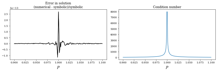
Example : rank and condition numbers -> numerical errors
p = sympy.symbols("p", positive=True)
A = sympy.Matrix([[1, sympy.sqrt(p)], [1, 1/sympy.sqrt(p)]])
b = sympy.Matrix([1, 2])
sympy.simplify(A.solve(b))
$\displaystyle \left[\begin{matrix}\frac{2 p - 1}{p - 1}\- \frac{\sqrt{p}}{p - 1}\end{matrix}\right]$
# Symbolic problem specification
p = sympy.symbols("p", positive=True)
A = sympy.Matrix([[1, sympy.sqrt(p)], [1, 1/sympy.sqrt(p)]])
b = sympy.Matrix([1, 2])

# Solve symbolically
x_sym_sol = A.solve(b)
x_sym_sol.simplify()
x_sym_sol
Acond = A.condition_number().simplify()

# Function for solving numerically
AA = lambda p: np.array([[1, np.sqrt(p)], [1, 1/np.sqrt(p)]])
bb = np.array([1, 2])
x_num_sol = lambda p: np.linalg.solve(AA(p), bb)

# Graph the difference between the symbolic (exact) and numerical results.
p_vec = np.linspace(0.9, 1.1, 200)

fig, axes = plt.subplots(1, 2, figsize=(12, 4))

for n in range(2):
    x_sym = np.array([x_sym_sol[n].subs(p, pp).evalf() for pp in p_vec])
    x_num = np.array([x_num_sol(pp)[n] for pp in p_vec])
    axes[0].plot(p_vec, (x_num - x_sym)/x_sym, 'k')
axes[0].set_title("Error in solution\n(numerical - symbolic)/symbolic")
axes[0].set_xlabel(r'$p$', fontsize=18)

axes[1].plot(p_vec, [Acond.subs(p, pp).evalf() for pp in p_vec])
axes[1].set_title("Condition number")
axes[1].set_xlabel(r'$p$', fontsize=18)

fig.tight_layout()
fig.savefig('ch5-linear-systems-condition-number.pdf')
Rectangular systems
Underdetermined
unknown = sympy.symbols("x, y, z")
A = sympy.Matrix([[1, 2, 3], [4, 5, 6]])
x = sympy.Matrix(unknown)
b = sympy.Matrix([7, 8])
AA = A * x - b
sympy.solve(A*x - b, unknown)
$\displaystyle \left{ x : z - \frac{19}{3}, \ y : \frac{20}{3} - 2 z\right}$
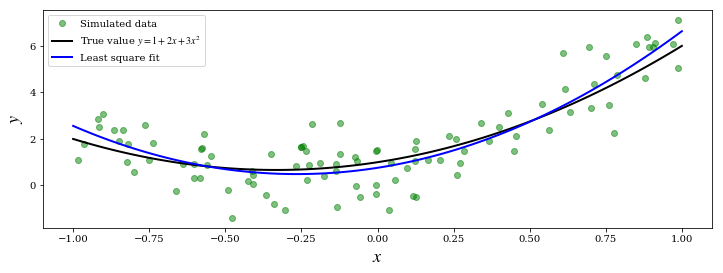
Overdetermined: least squares
np.random.seed(1234)

# define true model parameters
x = np.linspace(-1, 1, 100)
a, b, c = 1, 2, 3
y_exact = a + b * x + c * x**2

# simulate noisy data points
m = 100
X = 1 - 2 * np.random.rand(m)
Y = a + b * X + c * X**2 + np.random.randn(m)

# fit the data to the model using linear least square
A = np.vstack([X**0, X**1, X**2])  # see np.vander for alternative
sol, r, rank, sv = la.lstsq(A.T, Y)
y_fit = sol[0] + sol[1] * x + sol[2] * x**2
fig, ax = plt.subplots(figsize=(12, 4))

ax.plot(X, Y, 'go', alpha=0.5, label='Simulated data')
ax.plot(x, y_exact, 'k', lw=2, label='True value $y = 1 + 2x + 3x^2$')
ax.plot(x, y_fit, 'b', lw=2, label='Least square fit')
ax.set_xlabel(r"$x$", fontsize=18)
ax.set_ylabel(r"$y$", fontsize=18)
ax.legend(loc=2);

fig.savefig('ch5-linear-systems-least-square.pdf')
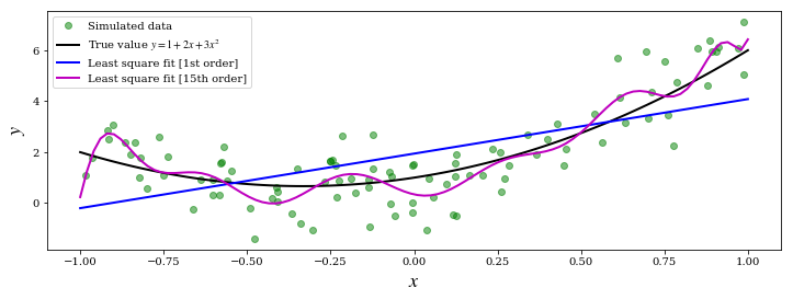
# fit the data to the model using linear least square:
# 1st order polynomial
A = np.vstack([X**n for n in range(2)])
sol, r, rank, sv = la.lstsq(A.T, Y)
y_fit1 = sum([s * x**n for n, s in enumerate(sol)])

# 15th order polynomial
A = np.vstack([X**n for n in range(16)])
sol, r, rank, sv = la.lstsq(A.T, Y)
y_fit15 = sum([s * x**n for n, s in enumerate(sol)])

fig, ax = plt.subplots(figsize=(12, 4))
ax.plot(X, Y, 'go', alpha=0.5, label='Simulated data')
ax.plot(x, y_exact, 'k', lw=2, label='True value $y = 1 + 2x + 3x^2$')
ax.plot(x, y_fit1, 'b', lw=2, label='Least square fit [1st order]')
ax.plot(x, y_fit15, 'm', lw=2, label='Least square fit [15th order]')
ax.set_xlabel(r"$x$", fontsize=18)
ax.set_ylabel(r"$y$", fontsize=18)
ax.legend(loc=2);

fig.savefig('ch5-linear-systems-least-square-2.pdf')
Eigenvalue problems
eps, delta = sympy.symbols("epsilon, delta")
H = sympy.Matrix([[eps, delta], [delta, -eps]])
H
$\displaystyle \left[\begin{matrix}\epsilon & \delta\\delta & - \epsilon\end{matrix}\right]$
eval1, eval2 = H.eigenvals()
eval1, eval2
$\displaystyle \left( - \sqrt{\delta^{2} + \epsilon^{2}}, \ \sqrt{\delta^{2} + \epsilon^{2}}\right)$
H.eigenvects()
$\displaystyle \left[ \left( - \sqrt{\delta^{2} + \epsilon^{2}}, \ 1, \ \left[ \left[\begin{matrix}- \frac{\delta}{\epsilon + \sqrt{\delta^{2} + \epsilon^{2}}}\1\end{matrix}\right]\right]\right), \ \left( \sqrt{\delta^{2} + \epsilon^{2}}, \ 1, \ \left[ \left[\begin{matrix}- \frac{\delta}{\epsilon - \sqrt{\delta^{2} + \epsilon^{2}}}\1\end{matrix}\right]\right]\right)\right]$
(eval1, _, evec1), (eval2, _, evec2) = H.eigenvects()
sympy.simplify(evec1[0].T * evec2[0])
$\displaystyle \left[\begin{matrix}0\end{matrix}\right]$
A = np.array([[1, 3, 5], [3, 5, 3], [5, 3, 9]])
A
array([[1, 3, 5],
       [3, 5, 3],
       [5, 3, 9]])
evals, evecs = la.eig(A)
evals
array([13.35310908+0.j, -1.75902942+0.j, 3.40592034+0.j])
evecs
array([[ 0.42663918,  0.90353276, -0.04009445],
       [ 0.43751227, -0.24498225, -0.8651975 ],
       [ 0.79155671, -0.35158534,  0.49982569]])
la.eigvalsh(A)
array([-1.75902942, 3.40592034, 13.35310908])
Nonlinear equations
Univariate
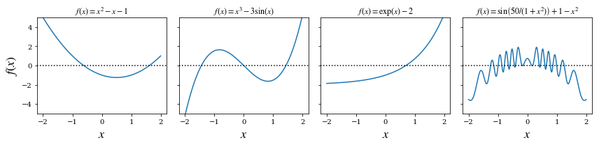
x = np.linspace(-2, 2, 1000)

# four examples of nonlinear functions
f1 = x**2 - x - 1
f2 = x**3 - 3 * np.sin(x)
f3 = np.exp(x) - 2
f4 = 1 - x**2 + np.sin(50 / (1 + x**2))

# plot each function
fig, axes = plt.subplots(1, 4, figsize=(12, 3), sharey=True)

for n, f in enumerate([f1, f2, f3, f4]):
    axes[n].plot(x, f, lw=1.5)
    axes[n].axhline(0, ls=':', color='k')
    axes[n].set_ylim(-5, 5)
    axes[n].set_xticks([-2, -1, 0, 1, 2])
    axes[n].set_xlabel(r'$x$', fontsize=18)

axes[0].set_ylabel(r'$f(x)$', fontsize=18)

titles = [r'$f(x)=x^2-x-1$', r'$f(x)=x^3-3\sin(x)$',
          r'$f(x)=\exp(x)-2$', r'$f(x)=\sin\left(50/(1+x^2)\right)+1-x^2$']
for n, title in enumerate(titles):
    axes[n].set_title(title)

fig.tight_layout()
fig.savefig('ch5-nonlinear-plot-equations.pdf')
Symbolic
x, a, b, c = sympy.symbols("x, a, b, c")
e = a + b*x + c*x**2
sol1, sol2 = sympy.solve(e, x)

sol1, sol2
$\displaystyle \left( \frac{- b + \sqrt{- 4 a c + b^{2}}}{2 c}, \ - \frac{b + \sqrt{- 4 a c + b^{2}}}{2 c}\right)$
e.subs(x, sol1).expand()
$\displaystyle 0$
e.subs(x, sol2).expand()
$\displaystyle 0$
e = a * sympy.cos(x) - b * sympy.sin(x)
sol1, sol2 = sympy.solve(e, x)

sol1, sol2
$\displaystyle \left( - 2 \operatorname{atan}{\left(\frac{b - \sqrt{a^{2} + b^{2}}}{a} \right)}, \ - 2 \operatorname{atan}{\left(\frac{b + \sqrt{a^{2} + b^{2}}}{a} \right)}\right)$
e.subs(x, sympy.atan(a/b))
$\displaystyle 0$
e.subs(x, sol1).simplify()
$\displaystyle 0$
e.subs(x, sol2).simplify()
$\displaystyle 0$
sympy.solve(sympy.sin(x)-x, x)
---------------------------------------------------------------------------

NotImplementedError                       Traceback (most recent call last)

<ipython-input-68-d3ec18de60c6> in <module>
----> 1 sympy.solve(sympy.sin(x)-x, x)


~/miniconda3/envs/py3.6/lib/python3.6/site-packages/sympy/solvers/solvers.py in solve(f, *symbols, **flags)
   1169     ###########################################################################
   1170     if bare_f:
-> 1171         solution = _solve(f[0], *symbols, **flags)
   1172     else:
   1173         solution = _solve_system(f, symbols, **flags)


~/miniconda3/envs/py3.6/lib/python3.6/site-packages/sympy/solvers/solvers.py in _solve(f, *symbols, **flags)
   1740
   1741     if result is False:
-> 1742         raise NotImplementedError('\n'.join([msg, not_impl_msg % f]))
   1743
   1744     if flags.get('simplify', True):


NotImplementedError: multiple generators [x, sin(x)]
No algorithms are implemented to solve equation -x + sin(x)
Bisection method
# define a function, desired tolerance and starting interval [a, b]
f = lambda x: np.exp(x) - 2
tol = 0.1
a, b = -2, 2
x = np.linspace(-2.1, 2.1, 1000)

# graph the function f
fig, ax = plt.subplots(1, 1, figsize=(12, 4))

ax.plot(x, f(x), lw=1.5)
ax.axhline(0, ls=':', color='k')
ax.set_xticks([-2, -1, 0, 1, 2])
ax.set_xlabel(r'$x$', fontsize=18)
ax.set_ylabel(r'$f(x)$', fontsize=18)

# find the root using the bisection method and visualize
# the steps in the method in the graph
fa, fb = f(a), f(b)

ax.plot(a, fa, 'ko')
ax.plot(b, fb, 'ko')
ax.text(a, fa + 0.5, r"$a$", ha='center', fontsize=18)
ax.text(b, fb + 0.5, r"$b$", ha='center', fontsize=18)

n = 1
while b - a > tol:
    m = a + (b - a)/2
    fm = f(m)

    ax.plot(m, fm, 'ko')
    ax.text(m, fm - 0.5, r"$m_%d$" % n, ha='center')
    n += 1

    if np.sign(fa) == np.sign(fm):
        a, fa = m, fm
    else:
        b, fb = m, fm

ax.plot(m, fm, 'r*', markersize=10)
ax.annotate("Root approximately at %.3f" % m,
            fontsize=14, family="serif",
            xy=(a, fm), xycoords='data',
            xytext=(-150, +50), textcoords='offset points',
            arrowprops=dict(arrowstyle="->", connectionstyle="arc3, rad=-.5"))

ax.set_title("Bisection method")

fig.tight_layout()
fig.savefig('ch5-nonlinear-bisection.pdf')
# define a function, desired tolerance and starting point xk
tol = 0.01
xk = 2

s_x = sympy.symbols("x")
s_f = sympy.exp(s_x) - 2

f = lambda x: sympy.lambdify(s_x, s_f, 'numpy')(x)
fp = lambda x: sympy.lambdify(s_x, sympy.diff(s_f, s_x), 'numpy')(x)

x = np.linspace(-1, 2.1, 1000)

# setup a graph for visualizing the root finding steps
fig, ax = plt.subplots(1, 1, figsize=(12,4))

ax.plot(x, f(x))
ax.axhline(0, ls=':', color='k')

# repeat Newton's method until convergence to the desired tolerance has been reached
n = 0
while f(xk) > tol:
    xk_new = xk - f(xk) / fp(xk)

    ax.plot([xk, xk], [0, f(xk)], color='k', ls=':')
    ax.plot(xk, f(xk), 'ko')
    ax.text(xk, -.5, r'$x_%d$' % n, ha='center')
    ax.plot([xk, xk_new], [f(xk), 0], 'k-')

    xk = xk_new
    n += 1

ax.plot(xk, f(xk), 'r*', markersize=15)
ax.annotate("Root approximately at %.3f" % xk,
            fontsize=14, family="serif",
            xy=(xk, f(xk)), xycoords='data',
            xytext=(-150, +50), textcoords='offset points',
            arrowprops=dict(arrowstyle="->", connectionstyle="arc3, rad=-.5"))

ax.set_title("Newton's method")
ax.set_xticks([-1, 0, 1, 2])
fig.tight_layout()
fig.savefig('ch5-nonlinear-newton.pdf')
scipy.optimize functions for root-finding
optimize.bisect(lambda x: np.exp(x) - 2, -2, 2)
$\displaystyle 0.6931471805601177$
optimize.newton(lambda x: np.exp(x) - 2, 2)
$\displaystyle 0.6931471805599455$
x_root_guess = 2
f = lambda x: np.exp(x) - 2
fprime = lambda x: np.exp(x)
optimize.newton(f, x_root_guess)
$\displaystyle 0.6931471805599455$
optimize.newton(f, x_root_guess, fprime=fprime)
$\displaystyle 0.6931471805599453$
optimize.brentq(lambda x: np.exp(x) - 2, -2, 2)
$\displaystyle 0.6931471805599453$
optimize.brenth(lambda x: np.exp(x) - 2, -2, 2)
$\displaystyle 0.6931471805599381$
optimize.ridder(lambda x: np.exp(x) - 2, -2, 2)
$\displaystyle 0.6931471805590396$
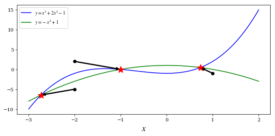
Multivariate
def f(x):
    return [x[1] - x[0]**3 - 2 * x[0]**2 + 1, x[1] + x[0]**2 - 1]
optimize.fsolve(f, [1, 1])
array([0.73205081, 0.46410162])
def f_jacobian(x):
    return [[-3*x[0]**2-4*x[0], 1], [2*x[0], 1]]
optimize.fsolve(f, [1, 1], fprime=f_jacobian)
array([0.73205081, 0.46410162])
x, y = sympy.symbols("x, y")

f_mat = sympy.Matrix([y - x**3 -2*x**2 + 1, y + x**2 - 1])
f_mat.jacobian(sympy.Matrix([x, y]))
$\displaystyle \left[\begin{matrix}- 3 x^{2} - 4 x & 1\2 x & 1\end{matrix}\right]$
#def f(x):
#    return [x[1] - x[0]**3 - 2 * x[0]**2 + 1, x[1] + x[0]**2 - 1]

x = np.linspace(-3, 2, 5000)
y1 = x**3 + 2 * x**2 -1
y2 = -x**2 + 1

fig, ax = plt.subplots(figsize=(8, 4))

ax.plot(x, y1, 'b', lw=1.5, label=r'$y = x^3 + 2x^2 - 1$')
ax.plot(x, y2, 'g', lw=1.5, label=r'$y = -x^2 + 1$')

x_guesses = [[-2, 2], [1, -1], [-2, -5]]
for x_guess in x_guesses:
    sol = optimize.fsolve(f, x_guess)
    ax.plot(sol[0], sol[1], 'r*', markersize=15)

    ax.plot(x_guess[0], x_guess[1], 'ko')
    ax.annotate("", xy=(sol[0], sol[1]), xytext=(x_guess[0], x_guess[1]),
                arrowprops=dict(arrowstyle="->", linewidth=2.5))

ax.legend(loc=0)
ax.set_xlabel(r'$x$', fontsize=18)
fig.tight_layout()
fig.savefig('ch5-nonlinear-system.pdf')
optimize.broyden2(f, x_guesses[1])
array([0.73205079, 0.46410162])
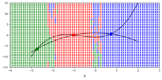
def f(x):
    return [x[1] - x[0]**3 - 2 * x[0]**2 + 1,
            x[1] + x[0]**2 - 1]

x = np.linspace(-3, 2, 5000)
y1 = x**3 + 2 * x**2 -1
y2 = -x**2 + 1

fig, ax = plt.subplots(figsize=(8, 4))

ax.plot(x, y1, 'k', lw=1.5, label=r'$y = x^3 + 2x^2 - 1$')
ax.plot(x, y2, 'k', lw=1.5, label=r'$y = -x^2 + 1$')

sol1 = optimize.fsolve(f, [-2,  2])
sol2 = optimize.fsolve(f, [ 1, -1])
sol3 = optimize.fsolve(f, [-2, -5])
sols = [sol1, sol2, sol3]
colors = ['r', 'b', 'g']
for idx, s in enumerate(sols):
    ax.plot(s[0], s[1], colors[idx]+'*', markersize=15)

for m in np.linspace(-4, 3, 80):
    for n in np.linspace(-15, 15, 40):
        x_guess = [m, n]
        sol = optimize.fsolve(f, x_guess)
        idx = (abs(sols - sol)**2).sum(axis=1).argmin()
        ax.plot(x_guess[0], x_guess[1], colors[idx]+'.')

ax.set_xlabel(r'$x$', fontsize=18)
ax.set_xlim(-4, 3)
ax.set_ylim(-15, 15)
fig.tight_layout()
fig.savefig('ch5-nonlinear-system-map.pdf')
/Users/rob/miniconda3/envs/py3.6/lib/python3.6/site-packages/scipy/optimize/minpack.py:162: RuntimeWarning: The iteration is not making good progress, as measured by the
  improvement from the last ten iterations.
  warnings.warn(msg, RuntimeWarning)
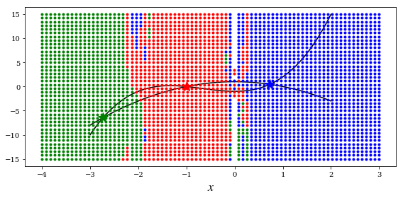
def f(x):
    return [x[1] - x[0]**3 - 2 * x[0]**2 + 1,
            x[1] + x[0]**2 - 1]

x = np.linspace(-3, 2, 5000)
y1 = x**3 + 2 * x**2 -1
y2 = -x**2 + 1

fig, ax = plt.subplots(figsize=(8, 4))

ax.plot(x, y1, 'k', lw=1.5, label=r'$y = x^3 + 2x^2 - 1$')
ax.plot(x, y2, 'k', lw=1.5, label=r'$y = -x^2 + 1$')

sol1 = optimize.fsolve(f, [-2,  2])
sol2 = optimize.fsolve(f, [ 1, -1])
sol3 = optimize.fsolve(f, [-2, -5])

for idx, s in enumerate([sol1, sol2, sol3]):
    ax.plot(s[0], s[1], colors[idx]+'*', markersize=15)

colors = ['r', 'b', 'g']
for m in np.linspace(-4, 3, 80):
    for n in np.linspace(-15, 15, 40):
        x_guess = [m, n]
        sol = optimize.fsolve(f, x_guess)

        for idx, s in enumerate([sol1, sol2, sol3]):
            if abs(s-sol).max() < 1e-8:
                # ax.plot(sol[0], sol[1], colors[idx]+'*', markersize=15)
                ax.plot(x_guess[0], x_guess[1], colors[idx]+'.')

ax.set_xlabel(r'$x$', fontsize=18)
fig.tight_layout()
fig.savefig('ch5-nonlinear-system-map.pdf')
Versions
%reload_ext version_information
%version_information sympy, scipy, numpy, matplotlib