Jupyter Snippet NP ch06-code-listing
Jupyter Snippet NP ch06-code-listing
Chapter 6: Optimization
Robert Johansson
Source code listings for Numerical Python - Scientific Computing and Data Science Applications with Numpy, SciPy and Matplotlib (ISBN 978-1-484242-45-2).
%matplotlib inline
import matplotlib.pyplot as plt
import matplotlib
matplotlib.rcParams['mathtext.fontset'] = 'stix'
matplotlib.rcParams['font.family'] = 'serif'
matplotlib.rcParams['font.sans-serif'] = 'stix'
import numpy as np
import sympy
sympy.init_printing()
from scipy import optimize
import cvxopt
from __future__ import division
Univariate
r, h = sympy.symbols("r, h")
Area = 2 * sympy.pi * r**2 + 2 * sympy.pi * r * h
Volume = sympy.pi * r**2 * h
h_r = sympy.solve(Volume - 1)[0]
Area_r = Area.subs(h_r)
rsol = sympy.solve(Area_r.diff(r))[0]
rsol
$$\frac{2^{\frac{2}{3}}}{2 \sqrt[3]{\pi}}$$
_.evalf()
$$0.541926070139289$$
# verify that the second derivative is positive, so that rsol is a minimum
Area_r.diff(r, 2).subs(r, rsol)
$$12 \pi$$
Area_r.subs(r, rsol)
$$3 \sqrt[3]{2} \sqrt[3]{\pi}$$
_.evalf()
$$5.53581044593209$$
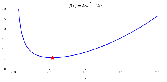
def f(r):
    return 2 * np.pi * r**2 + 2 / r
r_min = optimize.brent(f, brack=(0.1, 4))
r_min
$$0.541926077256$$
f(r_min)
$$5.53581044593$$
optimize.minimize_scalar(f, bracket=(0.1, 4))
     fun: 5.5358104459320856
    nfev: 19
     nit: 15
 success: True
       x: 0.54192607725571351
r = np.linspace(0, 2, 100)[1:]
fig, ax = plt.subplots(figsize=(8, 4))

ax.plot(r, f(r), lw=2, color='b')
ax.plot(r_min, f(r_min), 'r*', markersize=15)
ax.set_title(r"$f(r) = 2\pi r^2+2/r$", fontsize=18)
ax.set_xlabel(r"$r$", fontsize=18)
ax.set_xticks([0, 0.5, 1, 1.5, 2])
ax.set_ylim(0, 30)

fig.tight_layout()
fig.savefig('ch6-univariate-optimization-example.pdf')
Two-dimensional
x1, x2 = sympy.symbols("x_1, x_2")
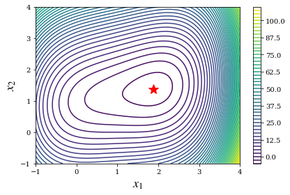
f_sym = (x1-1)**4 + 5 * (x2-1)**2 - 2*x1*x2
fprime_sym = [f_sym.diff(x_) for x_ in (x1, x2)]
# Gradient
sympy.Matrix(fprime_sym)
$$\left[\begin{matrix}- 2 x_{2} + 4 \left(x_{1} - 1\right)^{3}\- 2 x_{1} + 10 x_{2} - 10\end{matrix}\right]$$
fhess_sym = [[f_sym.diff(x1_, x2_) for x1_ in (x1, x2)] for x2_ in (x1, x2)]
# Hessian
sympy.Matrix(fhess_sym)
$$\left[\begin{matrix}12 \left(x_{1} - 1\right)^{2} & -2\-2 & 10\end{matrix}\right]$$
f_lmbda = sympy.lambdify((x1, x2), f_sym, 'numpy')
fprime_lmbda = sympy.lambdify((x1, x2), fprime_sym, 'numpy')
fhess_lmbda = sympy.lambdify((x1, x2), fhess_sym, 'numpy')
def func_XY_X_Y(f):
    """
    Wrapper for f(X) -> f(X[0], X[1])
    """
    return lambda X: np.array(f(X[0], X[1]))
f = func_XY_X_Y(f_lmbda)
fprime = func_XY_X_Y(fprime_lmbda)
fhess = func_XY_X_Y(fhess_lmbda)
X_opt = optimize.fmin_ncg(f, (0, 0), fprime=fprime, fhess=fhess)
Optimization terminated successfully.
         Current function value: -3.867223
         Iterations: 8
         Function evaluations: 10
         Gradient evaluations: 17
         Hessian evaluations: 8
X_opt
array([ 1.88292613, 1.37658523])
fig, ax = plt.subplots(figsize=(6, 4))
x_ = y_ = np.linspace(-1, 4, 100)
X, Y = np.meshgrid(x_, y_)
c = ax.contour(X, Y, f_lmbda(X, Y), 50)
ax.plot(X_opt[0], X_opt[1], 'r*', markersize=15)
ax.set_xlabel(r"$x_1$", fontsize=18)
ax.set_ylabel(r"$x_2$", fontsize=18)
plt.colorbar(c, ax=ax)
fig.tight_layout()
fig.savefig('ch6-examaple-two-dim.pdf');
Brute force search for initial point
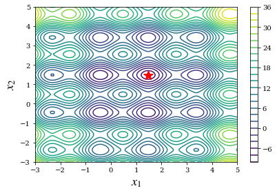
def f(X):
    x, y = X
    return (4 * np.sin(np.pi * x) + 6 * np.sin(np.pi * y)) + (x - 1)**2 + (y - 1)**2
x_start = optimize.brute(f, (slice(-3, 5, 0.5), slice(-3, 5, 0.5)), finish=None)
x_start
array([ 1.5, 1.5])
f(x_start)
$$-9.5$$
x_opt = optimize.fmin_bfgs(f, x_start)
Optimization terminated successfully.
         Current function value: -9.520229
         Iterations: 4
         Function evaluations: 28
         Gradient evaluations: 7
x_opt
array([ 1.47586906, 1.48365787])
f(x_opt)
$$-9.52022927306$$
def func_X_Y_to_XY(f, X, Y):
    s = np.shape(X)
    return f(np.vstack([X.ravel(), Y.ravel()])).reshape(*s)
fig, ax = plt.subplots(figsize=(6, 4))
x_ = y_ = np.linspace(-3, 5, 100)
X, Y = np.meshgrid(x_, y_)
c = ax.contour(X, Y, func_X_Y_to_XY(f, X, Y), 25)
ax.plot(x_opt[0], x_opt[1], 'r*', markersize=15)
ax.set_xlabel(r"$x_1$", fontsize=18)
ax.set_ylabel(r"$x_2$", fontsize=18)
plt.colorbar(c, ax=ax)
fig.tight_layout()
fig.savefig('ch6-example-2d-many-minima.pdf');
Nonlinear least square
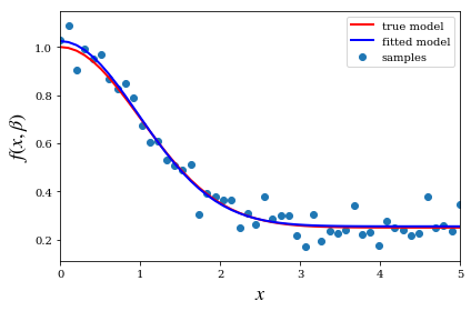
def f(x, beta0, beta1, beta2):
    return beta0 + beta1 * np.exp(-beta2 * x**2)
beta = (0.25, 0.75, 0.5)
xdata = np.linspace(0, 5, 50)
y = f(xdata, *beta)
ydata = y + 0.05 * np.random.randn(len(xdata))
def g(beta):
    return ydata - f(xdata, *beta)
beta_start = (1, 1, 1)
beta_opt, beta_cov = optimize.leastsq(g, beta_start)
beta_opt
array([ 0.25498249, 0.7693897 , 0.52778771])
fig, ax = plt.subplots()

ax.scatter(xdata, ydata, label="samples")
ax.plot(xdata, y, 'r', lw=2, label="true model")
ax.plot(xdata, f(xdata, *beta_opt), 'b', lw=2, label="fitted model")
ax.set_xlim(0, 5)
ax.set_xlabel(r"$x$", fontsize=18)
ax.set_ylabel(r"$f(x, \beta)$", fontsize=18)
ax.legend()
fig.tight_layout()
fig.savefig('ch6-nonlinear-least-square.pdf')
beta_opt, beta_cov = optimize.curve_fit(f, xdata, ydata)
beta_opt
array([ 0.25498249, 0.7693897 , 0.52778771])
Constrained optimization
Bounds
def f(X):
    x, y = X
    return (x-1)**2 + (y-1)**2
x_opt = optimize.minimize(f, [0, 0], method='BFGS').x
bnd_x1, bnd_x2 = (2, 3), (0, 2)
x_cons_opt = optimize.minimize(f, [0, 0], method='L-BFGS-B', bounds=[bnd_x1, bnd_x2]).x
fig, ax = plt.subplots(figsize=(6, 4))
x_ = y_ = np.linspace(-1, 3, 100)
X, Y = np.meshgrid(x_, y_)
c = ax.contour(X, Y, func_X_Y_to_XY(f, X, Y), 50)
ax.plot(x_opt[0], x_opt[1], 'b*', markersize=15)
ax.plot(x_cons_opt[0], x_cons_opt[1], 'r*', markersize=15)
bound_rect = plt.Rectangle((bnd_x1[0], bnd_x2[0]),
                           bnd_x1[1] - bnd_x1[0], bnd_x2[1] - bnd_x2[0],
                           facecolor="grey")
ax.add_patch(bound_rect)
ax.set_xlabel(r"$x_1$", fontsize=18)
ax.set_ylabel(r"$x_2$", fontsize=18)
plt.colorbar(c, ax=ax)

fig.tight_layout()
fig.savefig('ch6-example-constraint-bound.pdf');
Lagrange multiplier
x = x1, x2, x3, l = sympy.symbols("x_1, x_2, x_3, lambda")
f = x1 * x2 * x3
g = 2 * (x1 * x2 + x2 * x3 + x3 * x1) - 1
L = f + l * g
grad_L = [sympy.diff(L, x_) for x_ in x]
sols = sympy.solve(grad_L)
sols
g.subs(sols[0])
f.subs(sols[0])
def f(X):
    return -X[0] * X[1] * X[2]
def g(X):
    return 2 * (X[0]*X[1] + X[1] * X[2] + X[2] * X[0]) - 1
constraints = [dict(type='eq', fun=g)]
result = optimize.minimize(f, [0.5, 1, 1.5], method='SLSQP', constraints=constraints)
result
result.x
Inequality constraints
def f(X):
    return (X[0] - 1)**2 + (X[1] - 1)**2

def g(X):
    return X[1] - 1.75 - (X[0] - 0.75)**4
%time x_opt = optimize.minimize(f, (0, 0), method='BFGS').x
constraints = [dict(type='ineq', fun=g)]
%time x_cons_opt = optimize.minimize(f, (0, 0), method='SLSQP', constraints=constraints).x
%time x_cons_opt = optimize.minimize(f, (0, 0), method='COBYLA', constraints=constraints).x
fig, ax = plt.subplots(figsize=(6, 4))
x_ = y_ = np.linspace(-1, 3, 100)
X, Y = np.meshgrid(x_, y_)
c = ax.contour(X, Y, func_X_Y_to_XY(f, X, Y), 50)
ax.plot(x_opt[0], x_opt[1], 'b*', markersize=15)

ax.plot(x_, 1.75 + (x_-0.75)**4, 'k-', markersize=15)
ax.fill_between(x_, 1.75 + (x_-0.75)**4, 3, color="grey")
ax.plot(x_cons_opt[0], x_cons_opt[1], 'r*', markersize=15)

ax.set_ylim(-1, 3)
ax.set_xlabel(r"$x_0$", fontsize=18)
ax.set_ylabel(r"$x_1$", fontsize=18)
plt.colorbar(c, ax=ax)

fig.tight_layout()
fig.savefig('ch6-example-constraint-inequality.pdf');
Linear programming
c = np.array([-1.0, 2.0, -3.0])

A = np.array([[ 1.0, 1.0, 0.0],
              [-1.0, 3.0, 0.0],
              [ 0.0, -1.0, 1.0]])

b = np.array([1.0, 2.0, 3.0])
A_ = cvxopt.matrix(A)
b_ = cvxopt.matrix(b)
c_ = cvxopt.matrix(c)
sol = cvxopt.solvers.lp(c_, A_, b_)
x = np.array(sol['x'])
x
sol
sol['primal objective']
Quandratic problem with cvxopt
Quadratic problem formulation:
$\min \frac{1}{2}x^TPx + q^T x$
$G x \leq h$
For example, let’s solve the problem
min $f(x_1, x_2) = (x_1 - 1)^2 + (x_2 - 1)^2 =$
$x_1^2 -2x_1 + 1 + x_2^2 - 2x_2 + 1 = $
$x_1^2 + x_2^2 - 2x_1 - 2x_2 + 2 =$
$= \frac{1}{2} x^T P x - q^T x + 2$
and
$\frac{3}{4} x_1 + x_2 \geq 3$, $x_1 \geq 0$
where
$P = 2 [[1, 0], [0, 1]]$ and $q = [-2, -2]$
and
$G = [[-3/4, -1], [-1, 0]]$ and $h = [-3, 0]$
from cvxopt import matrix, solvers

P = 2 * np.array([[1.0, 0.0],
                  [0.0, 1.0]])
q = np.array([-2.0, -2.0])

G = np.array([[-0.75, -1.0],
              [-1.0,  0.0]])

h = np.array([-3.0, 0.0])
_P = cvxopt.matrix(P)
_q = cvxopt.matrix(q)
_G = cvxopt.matrix(G)
_h = cvxopt.matrix(h)
%time sol = solvers.qp(_P, _q, _G, _h)
# sol
x = sol['x']
x = np.array(x)
sol['primal objective'] + 2
fig, ax = plt.subplots(figsize=(6, 4))
x_ = y_ = np.linspace(-1, 3, 100)
X, Y = np.meshgrid(x_, y_)
c = ax.contour(X, Y, func_X_Y_to_XY(f, X, Y), 50)


y_ = (h[0] - G[0, 0] * x_)/G[0, 1]
angle = -np.arctan((y_[mask][0] - y_[mask][-1]) / (x_[mask][-1]- x_[mask][0])) * 180 / np.pi
mask = y_ < 3
ax.plot(x_, y_, 'k')
ax.add_patch(plt.Rectangle((0, 3), 4, 3, angle=angle, facecolor="grey"))

ax.plot(x_opt[0], x_opt[1], 'b*', markersize=15)
ax.plot(x[0], x[1], 'r*', markersize=15)

ax.set_ylim(-1, 3)
ax.set_xlim(-1, 3)
ax.set_xlabel(r"$x_1$", fontsize=18)
ax.set_ylabel(r"$x_2$", fontsize=18)
plt.colorbar(c, ax=ax)

fig.tight_layout()
fig.savefig('ch6-example-quadratic-problem-constraint-inequality.pdf');
Arbitrary function callback API
from cvxopt import modeling
x1 = modeling.variable(1, "x1")
x2 = modeling.variable(1, "x2")
x1 * x2 + x2
help(modeling)
help(solvers)
help(solvers.cp)
CVXPY

cvxpy.org
Versions
%reload_ext version_information
%version_information numpy, scipy, cvxopt, sympy, matplotlib